Data Handling and Analysis
This tutorial gives an in depth overview of the PhotometryData class. PhotometryData is the main container for trial-wise photometry signals after an experiment has been processed and split into windows.
PhotometryData is built around an AnnData object. You do not need to know the ins and outs of AnnData to use this package, but it helps to understand the layout:
-
X(np.ndarray): contains the main signal matrix with shape(n_trials, n_timepoints). -
obs(pd.DataFrame): contains a table of metadata with shape(n_trials, n_observations). -
var(pd.DataFrame): contains one row of metadata for each timepoint. In this package, its main use is to hold the values of the timepoint in the columnt. -
layers(np.ndarray): can store extra signal matrices of the same shape ofX, such as standard deviations after averaging. -
uns(dict): stores unstructured metadata about the dataset, subject, processing choices, and file provenance.
Setup
First we need to import the packages used in this tutorial.
import numpy as np
import pandas as pd
from plotnine import * # type: ignore

from PhoPro import PhotometryData
1. Loading Trial-wise Data
Most workflows create PhotometryData by calling PhotometryExperiment.extract_trial_data() after preprocessing an experiment. The result can then be savedas an .h5ad file. The zarr format is also supported, but the .h5ad is more straight-forward.
Photometry dataset with 20 trials, 1598 timepoints, and 5 observations.
The string representation gives a compact summary of how many trials, timepoints, and observation columns are available.
The underlying trial matrix is available through .X, where rows are trials and columns are timepoints.
(20, 1598)
The time axis is available through .ts. PhotometryData also estimates .freq and .dt from this time axis.
[-8.        -7.9899901 -7.9799802 -7.9699703 -7.9599604]
[7.9457707 7.9557806 7.9657905 7.9758004 7.9858103]
94.07852623904556
0.010629418210262826
2. Understanding obs, var, uns, and layers
The obs dataframe is where trial-level metadata lives. In this example, each row is a trial and the columns contain event times relative to the window. A value of NaN in an event column represents that the event does not within that trial.
| trial_num | trial_cue | lever1 | lever2 | shock | |
|---|---|---|---|---|---|
| 0 | 1 | -3.52 | 0.0 | NaN | NaN |
| 1 | 2 | -2.71 | 0.0 | NaN | 1.22 |
| 2 | 3 | 0.00 | NaN | NaN | NaN |
| 3 | 4 | -3.94 | 0.0 | NaN | NaN |
| 4 | 5 | -3.79 | 0.0 | NaN | NaN |
The var dataframe is across the timepoint axis. With the t containing the value of the time points.
| t | |
|---|---|
| 0 | -8.00000 |
| 1 | -7.98999 |
| 2 | -7.97998 |
| 3 | -7.96997 |
| 4 | -7.95996 |
The uns dictionary stores metadata that applies to the whole dataset. If the trial data came from PhotometryExperiment.extract_trial_data(), uns is automatically populated with the experiment's metadata.
{'age': 'young',
 'correction_method': 'dF/F',
 'invalid_windows': None,
 'reference_fit': {'coeffs': array([-0.00458822,  1.24991004]),
  'r2_val': 0.9990778344806817,
  'type': 'isosbestic'},
 'sex': 'male',
 'source': 'data/experiments/example_experiment.csv',
 'subject': 'animal_1'}
Layers store additional matrices with the same shape as X. This example starts without extra layers, but later we will create layers by collapsing trials. Layers can be easily accessed with the get_layers method.
[]
3. Constructing PhotometryData From Arrays
PhotometryData objects can also be built directly from arrays. This is useful when importing data from another package, writing tests, or creating small examples.
rng = np.random.default_rng(1)
time_points = np.linspace(-2, 4, 301)

obs = pd.DataFrame({
    'trial_num': np.arange(1, 7),
    'condition': ['A', 'A', 'A', 'B', 'B', 'B'],
    'cue': np.zeros(6),
})

signal = rng.normal(0, 0.05, size=(6, time_points.size))
signal += np.exp(-0.5 * ((time_points - 1.0) / 0.25) ** 2)
signal[obs['condition'].eq('B')] *= 1.4

synthetic = PhotometryData.from_arrays(
    obs=obs,
    data=signal,
    time_points=time_points,
    metadata={'source': 'synthetic example'},
)

synthetic
Photometry dataset with 6 trials, 301 timepoints, and 3 observations.
4. Filtering and Adding Metadata
filter_rows subsets trials and returns a new object by default. With inplace=True, the object will be modified in place and None will be returned. Often you will construct a trial selection from the values in obs.
Photometry dataset with 9 trials, 1598 timepoints, and 5 observations.
mutate_obs creates a copy and adds or replaces observation columns. Values can be arrays, scalars, or functions that receive the copied PhotometryData object.
annotated = data.mutate_obs(
    has_lever = lambda d: d.obs['lever1'].notna(),
    has_shock = lambda d: d.obs['shock'].notna(),
    trial_epoch = lambda d: np.where(d.obs['trial_num'] <= 10, 'early', 'late'),
)

annotated.obs.head()
| trial_num | trial_cue | lever1 | lever2 | shock | has_lever | has_shock | trial_epoch | |
|---|---|---|---|---|---|---|---|---|
| 0 | 1 | -3.52 | 0.0 | NaN | NaN | True | False | early |
| 1 | 2 | -2.71 | 0.0 | NaN | 1.22 | True | True | early |
| 2 | 3 | 0.00 | NaN | NaN | NaN | False | False | early |
| 3 | 4 | -3.94 | 0.0 | NaN | NaN | True | False | early |
| 4 | 5 | -3.79 | 0.0 | NaN | NaN | True | False | early |
You can modify the obs table directly, or use add_obs_columns and add_metadata to modify the object directly. The latter are useful for adding information from dictionaries, such as annotation files.
| trial_num | trial_cue | lever1 | lever2 | shock | subject | |
|---|---|---|---|---|---|---|
| 0 | 1 | -3.52 | 0.0 | NaN | NaN | animal_1 |
| 1 | 2 | -2.71 | 0.0 | NaN | 1.22 | animal_1 |
| 2 | 3 | 0.00 | NaN | NaN | NaN | animal_1 |
| 3 | 4 | -3.94 | 0.0 | NaN | NaN | animal_1 |
| 4 | 5 | -3.79 | 0.0 | NaN | NaN | animal_1 |
with_extra.add_obs_columns({
    'session': 'example_session',
    'cohort': 'tutorial',
})

with_extra.add_metadata({
    'tutorial_note': 'added during Handling Data tutorial',
})

with_extra.obs[['session', 'cohort']].head()
| session | cohort | |
|---|---|---|
| 0 | example_session | tutorial |
| 1 | example_session | tutorial |
| 2 | example_session | tutorial |
| 3 | example_session | tutorial |
| 4 | example_session | tutorial |
Columns can be removed with drop_obs_columns.
| trial_num | trial_cue | lever1 | lever2 | shock | subject | session | |
|---|---|---|---|---|---|---|---|
| 0 | 1 | -3.52 | 0.0 | NaN | NaN | animal_1 | example_session |
| 1 | 2 | -2.71 | 0.0 | NaN | 1.22 | animal_1 | example_session |
| 2 | 3 | 0.00 | NaN | NaN | NaN | animal_1 | example_session |
| 3 | 4 | -3.94 | 0.0 | NaN | NaN | animal_1 | example_session |
| 4 | 5 | -3.79 | 0.0 | NaN | NaN | animal_1 | example_session |
5. Plotting Trials
plot_trials converts trial data to a long dataframe and passes it to the utils.graphing helper module. It returns a ggplot object, so you can add plotnine layers, labels, and themes.
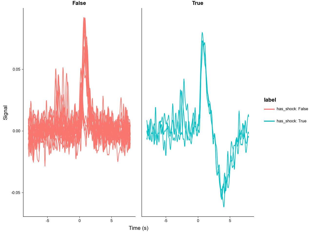
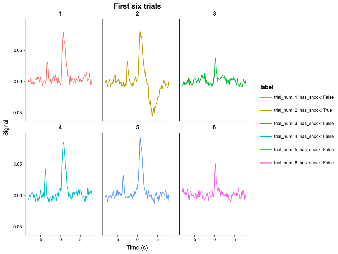
Use sel to plot a subset of trials. label_with controls legend labels and group_on controls line grouping.
p = annotated.plot_trials(
    sel=np.arange(6),
    label_with=['trial_num', 'has_shock'],
    group_on='trial_num',
    downsample=4,
)

p + labs(title='First six trials')
6. Downsampling
Downsampling is helpful for plotting, exporting, and reducing memory use. downsample returns a new PhotometryData object with fewer timepoints.
(20, 1598)
(20, 159)
[-7.95495545 -7.85485645 -7.75475745 -7.65465845 -7.55455945]
Two methods are supported. method='mean' downsamples using mean pooling while method='resample' uses scipy.signal.resample_ploy to downsample and accepts options such as window and padtype. 'resample' is generally more rigorious, but 'mean' is simpler and faster.
Photometry dataset with 20 trials, 200 timepoints, and 5 observations.
7. Averaging Trials
collapse summarizes trials by group. The primary aggregation (mean by default) becomes the new X matrix, and any additional metrics become layers. Passed data_cols undergo the same aggregation (including additional metrics) and are passed down to the new object.
collapsed = annotated.collapse(
    group_on='has_shock',
    method=np.nanmean,
    metrics={'std': np.nanstd, 'sem': lambda x, axis: np.nanstd(x, axis=axis) / np.sqrt(x.shape[axis])},
    data_cols=['trial_cue'],
    count_col='n',
)

collapsed.obs
| has_shock | n | trial_cue | trial_cue_std | trial_cue_sem | |
|---|---|---|---|---|---|
| 0 | False | 17 | -2.254706 | 1.541745 | 0.373928 |
| 1 | True | 3 | -2.680000 | 0.225536 | 0.130213 |
The collapsed object now has one row per aggregated group and the same time axis as the original data.
(2, 1598)
['std', 'sem']
Because the extra metrics are stored as layers, they can be used as error ribbons in plot_trials.
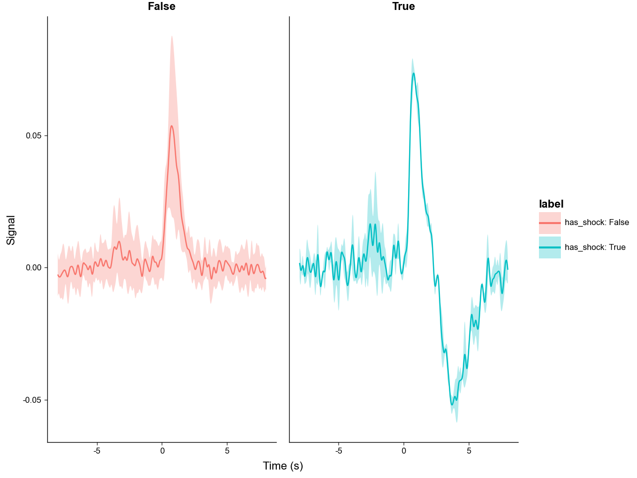
If group_on=None (default), all trials are collapsed into one average trace.
Photometry dataset with 1 trials, 1598 timepoints, and 1 observations.
8. Re-windowing Around Events
window creates a new PhotometryData object by slicing or interpolating each trial around a center time. Centers can be a scalar, an array, or the name of an obs column.
A scalar center is broadcast to all trials. This example keeps the interval from 1 second before time 0 to 3 seconds after time 0.
post_cue = data.window(
    centers=0.0,
    bounds=(-1, 3),
)

print(post_cue.X.shape)
print(post_cue.ts[:5])
print(post_cue.ts[-5:])
(20, 376)
[-0.99916531 -0.98853589 -0.97790648 -0.96727706 -0.95664764]
[2.94434884 2.95497826 2.96560768 2.9762371  2.98686652]
When event_cols are provided, those event times are re-centered relative to each window center. For example, after centering on shock, the shock column is zero for trials that contain shocks.
shock_trials = data.filter_rows(data.obs['shock'].notna())

shock_centered = shock_trials.window(
    centers='shock',
    bounds=(-2, 4),
    event_cols=['trial_cue', 'lever1', 'lever2', 'shock'],
)

shock_centered.obs[['trial_num', 'trial_cue', 'lever1', 'lever2', 'shock']].head()
| trial_num | trial_cue | lever1 | lever2 | shock | |
|---|---|---|---|---|---|
| 0 | 2 | -3.933891 | -1.221208 | NaN | 0.0 |
| 1 | 8 | -3.573534 | -1.181168 | NaN | 0.0 |
| 2 | 20 | -4.404356 | -1.461445 | NaN | 0.0 |
The default strategy='nearest' rounds windows to sampled timepoints. Use strategy='interp' to interpolate every trial onto an exact centered time grid.
nearest_window = shock_trials.window(
    centers='shock',
    bounds=(-1, 2),
    strategy='nearest',
)

interp_window = shock_trials.window(
    centers='shock',
    bounds=(-1, 2),
    strategy='interp',
)

print(nearest_window.ts[:5])
print(interp_window.ts[:5])
[-0.99916531 -0.98853589 -0.97790648 -0.96727706 -0.95664764]
[-1.         -0.98937058 -0.97874116 -0.96811175 -0.95748233]
If you have windows that extend outside the available time range, they will be default raise an error (invalid_window_policy='error'). Set invalid_window_policy='drop' to remove those trials instead.
valid_only = data.window(
    centers='shock',
    bounds=(-4, 4),
    event_cols=['shock'],
    invalid_window_policy='drop',
    verbose=True,
)

valid_only
Photometry dataset with 20 trials, 753 timepoints, and 5 observations.
9. Signal Features
PhotometryData includes a few analysis function for analyzing signals. difference calculates discrete differences along the time axis.
first_difference = data.difference(n=1)
second_difference = data.difference(n=2)

print(first_difference.shape)
print(second_difference.shape)
(20, 1598)
(20, 1598)
area_under_curve integrates each trial over time. By default it uses the whole trace. But, you can also pass the same arguements as the window function to integrate over a specified window. A transformation can also be passed when you want a specific feature, such as positive area only.
full_auc = data.area_under_curve()

response_auc = data.area_under_curve(
    centers=0.0,
    bounds=(0, 3),
    transformation=lambda x: np.maximum(x, 0),
)

print(full_auc[:5])
print(response_auc[:5])
[ 0.12073882 -0.02983236  0.02391584  0.09828795  0.1060965 ]
[0.0851429  0.09229777 0.02921103 0.09070887 0.09992221]
These per-trial values are best held in obs for trial-alignment, statistical analysis, and plotting.
features = annotated.mutate_obs(
    response_auc=response_auc,
    peak_value=lambda d: np.nanmax(d.X[:, (d.ts >= 0) & (d.ts <= 3)], axis=1),
)

features.obs.head()
| trial_num | trial_cue | lever1 | lever2 | shock | has_lever | has_shock | trial_epoch | response_auc | peak_value | |
|---|---|---|---|---|---|---|---|---|---|---|
| 0 | 1 | -3.52 | 0.0 | NaN | NaN | True | False | early | 0.085143 | 0.078496 |
| 1 | 2 | -2.71 | 0.0 | NaN | 1.22 | True | True | early | 0.092298 | 0.080037 |
| 2 | 3 | 0.00 | NaN | NaN | NaN | False | False | early | 0.029211 | 0.038073 |
| 3 | 4 | -3.94 | 0.0 | NaN | NaN | True | False | early | 0.090709 | 0.085493 |
| 4 | 5 | -3.79 | 0.0 | NaN | NaN | True | False | early | 0.099922 | 0.092526 |
10. Peak Detection
For event-like signals, PhotometryData can detect peaks using static or rolling thresholds (with more peak detection methods in the works). The static detector estimates one threshold per trial, while the rolling detector estimates a threshold that changes over time. All peak detection methods return a PeakResult object with an underlying pandas DataFrame df.
static_peaks = data.detect_peaks_static_threshold(
    center_method='median',
    scale_method='mad',
    test_magnitude=3,
    min_distance_sec=0.25,
    direction='positive',
)

static_peaks
    trial_idx direction  start_idx  stop_idx  start_time  stop_time  \
0           0  positive        457       496   -3.425476  -3.035090
1           0  positive        829       971    0.298207   1.719613
2           1  positive        538       565   -2.614674  -2.344406
3           1  positive        828       968    0.288197   1.689583
4           2  positive        808       845    0.087999   0.458365
5           3  positive        413       444   -3.865911  -3.555604
6           3  positive        828       959    0.288197   1.599494
7           4  positive        429       468   -3.705753  -3.315367
8           4  positive        811       961    0.118029   1.619514
9           5  positive        800       862    0.007920   0.628534
10          6  positive        459       482   -3.405456  -3.175228
11          6  positive        834       927    0.348257   1.279177
12          7  positive        579       586   -2.204268  -2.134199
13          7  positive        845       928    0.458365   1.289187
14          8  positive        519       532   -2.804862  -2.674733
15          8  positive        850       939    0.508415   1.399296
16          9  positive        606       629   -1.934001  -1.703773
17          9  positive        852       964    0.528435   1.649544
18         10  positive        587       610   -2.124189  -1.893961
19         10  positive        842       943    0.428336   1.439336
20         11  positive        822       842    0.228138   0.428336
21         12  positive        475       496   -3.245298  -3.035090
22         12  positive        835       958    0.358266   1.589484
23         13  positive        801       851    0.017930   0.518425
24         14  positive        462       486   -3.375426  -3.135189
25         14  positive        829       947    0.298207   1.479375
26         15  positive        419       443   -3.805852  -3.565614
27         15  positive        830       968    0.308217   1.689583
28         16  positive        842       934    0.428336   1.349247
29         17  positive        534       554   -2.654713  -2.454515
30         17  positive        844       938    0.448356   1.389286
31         18  positive        814       835    0.148059   0.358266
32         18  positive       1165      1170    3.661533   3.711583
33         19  positive        846       930    0.468375   1.309207

    peak_baseline  peak_idx  peak_time  peak_value    height  prominence  \
0        0.002853       472  -3.275327    0.031528  0.028675    0.012319
1        0.002853       874   0.748653    0.078496  0.075642    0.059553
2       -0.002691       548  -2.514575    0.032898  0.035589    0.010267
3       -0.002691       868   0.688593    0.080037  0.082727    0.057021
4        0.001090       823   0.238148    0.038073  0.036983    0.017613
5        0.001132       427  -3.725773    0.042679  0.041547    0.019555
6        0.001132       879   0.798702    0.085493  0.084362    0.061700
7        0.000807       447  -3.525575    0.032762  0.031954    0.015484
8        0.000807       869   0.698603    0.092526  0.091719    0.075306
9        0.001130       822   0.228138    0.051094  0.049963    0.034170
10       0.002188       470  -3.295347    0.046756  0.044568    0.016039
11       0.002188       883   0.838742    0.066248  0.064060    0.037436
12      -0.000551       582  -2.174238    0.042425  0.042976    0.001526
13      -0.000551       880   0.808712    0.073714  0.074265    0.032445
14       0.000891       524  -2.754812    0.029438  0.028547    0.001890
15       0.000891       864   0.648554    0.054395  0.053504    0.024619
16       0.002851       617  -1.823892    0.039867  0.037016    0.010210
17       0.002851       903   1.038940    0.067964  0.065113    0.039152
18       0.002979       599  -2.004070    0.047454  0.044476    0.013117
19       0.002979       886   0.868771    0.091915  0.088936    0.059158
20      -0.001399       832   0.328237    0.034185  0.035584    0.007257
21       0.000255       483  -3.165218    0.037539  0.037284    0.007183
22       0.000255       879   0.798702    0.087560  0.087306    0.057141
23       0.001309       825   0.258167    0.048643  0.047335    0.022339
24       0.001195       474  -3.255307    0.045625  0.044431    0.017138
25       0.001195       873   0.738643    0.068820  0.067625    0.039886
26       0.003035       430  -3.695743    0.051367  0.048332    0.018218
27       0.003035       876   0.768672    0.091255  0.088220    0.059404
28       0.000873       869   0.698603    0.088774  0.087902    0.053669
29      -0.001562       543  -2.564624    0.052014  0.053576    0.013218
30      -0.001562       893   0.938841    0.069969  0.071531    0.033465
31       0.000325       825   0.258167    0.040077  0.039752    0.011519
32       0.000325      1168   3.691563    0.028695  0.028370    0.000878
33      -0.001925       865   0.658563    0.073393  0.075318    0.029174

    duration     width      area
0   0.390386  0.390386  0.009525
1   1.421406  0.930921  0.068036
2   0.270267  0.270267  0.008408
3   1.401386  1.081069  0.081566
4   0.370366  0.370366  0.011134
5   0.310307  0.310307  0.010621
6   1.311297  0.930921  0.075315
7   0.390386  0.390386  0.010172
8   1.501485  0.940931  0.084956
9   0.620614  0.380376  0.020048
10  0.230228  0.230228  0.008808
11  0.930921  0.840832  0.044782
12  0.070069  0.070069  0.002974
13  0.830822  0.830822  0.050607
14  0.130129  0.130129  0.003612
15  0.890881  0.860851  0.035873
16  0.230228  0.230228  0.007701
17  1.121109  0.660653  0.047047
18  0.230228  0.230228  0.009146
19  1.011000  0.890881  0.067008
20  0.200198  0.200198  0.006603
21  0.210208  0.210208  0.007202
22  1.231218  0.970960  0.075023
23  0.500495  0.500495  0.019596
24  0.240238  0.240238  0.009170
25  1.181168  0.780772  0.054442
26  0.240238  0.240238  0.010001
27  1.381366  0.850841  0.079467
28  0.920911  0.770762  0.057605
29  0.200198  0.200198  0.009733
30  0.940931  0.670663  0.045401
31  0.210208  0.210208  0.007459
32  0.050050  0.050050  0.001401
33  0.840832  0.840832  0.053288
Use a baseline window when the detection threshold should be estimated from a specific period instead of the whole trial.
baseline = data.window(
    centers=0.0,
    bounds=(-5, -1),
    invalid_window_policy='drop',
)

baseline_peaks = data.detect_peaks_static_threshold(
    baselines=baseline.X,
    test_magnitude=3,
    direction='positive',
)

baseline_peaks
    trial_idx direction  start_idx  stop_idx  start_time  stop_time  \
0           0  positive        456       497   -3.435486  -3.025080
1           0  positive        829       973    0.298207   1.739633
2           1  positive        239       247   -5.607634  -5.527555
3           1  positive        533       585   -2.664723  -2.144209
4           1  positive        821      1003    0.218128   2.039930
5           2  positive        808       846    0.087999   0.468375
6           3  positive        408       452   -3.915961  -3.475525
7           3  positive        789       803   -0.102189   0.037950
8           3  positive        821       986    0.218128   1.869761
9           3  positive       1479      1490    6.804642   6.914751
10          4  positive        427       472   -3.725773  -3.275327
11          4  positive        805       966    0.057970   1.669563
12          5  positive        799       865   -0.002090   0.658563
13          6  positive        463       477   -3.365416  -3.225278
14          6  positive        840       915    0.408316   1.159059
15          7  positive        574       593   -2.254317  -2.064129
16          7  positive        841       934    0.418326   1.349247
17          8  positive        518       536   -2.814872  -2.634694
18          8  positive        849       943    0.498405   1.439336
19          9  positive        602       634   -1.974040  -1.653723
20          9  positive        728       735   -0.712793  -0.642723
21          9  positive        844       977    0.448356   1.779672
22         10  positive        589       609   -2.104169  -1.903971
23         10  positive        844       941    0.448356   1.419316
24         11  positive        818       846    0.188098   0.468375
25         12  positive        478       489   -3.215268  -3.105159
26         12  positive        839       952    0.398306   1.529425
27         13  positive        801       852    0.017930   0.528435
28         14  positive        462       486   -3.375426  -3.135189
29         14  positive        829       947    0.298207   1.479375
30         15  positive        419       444   -3.805852  -3.555604
31         15  positive        830       969    0.308217   1.699593
32         16  positive        841       937    0.418326   1.379276
33         17  positive        534       553   -2.654713  -2.464525
34         17  positive        847       908    0.478385   1.088989
35         17  positive        929       936    1.299197   1.369266
36         18  positive        280       291   -5.197228  -5.087119
37         18  positive        810       839    0.108019   0.398306
38         18  positive       1160      1175    3.611484   3.761632
39         18  positive       1243      1248    4.442306   4.492355
40         19  positive        526       531   -2.734793  -2.684743
41         19  positive        843       938    0.438346   1.389286

    peak_baseline  peak_idx  peak_time  peak_value    height  prominence  \
0        0.002422       472  -3.275327    0.031528  0.029106    0.013885
1        0.002422       874   0.748653    0.078496  0.076074    0.059662
2       -0.003018       243  -5.567594    0.011618  0.014636    0.000958
3       -0.003018       548  -2.514575    0.032898  0.035916    0.020697
4       -0.003018       868   0.688593    0.080037  0.083055    0.069015
5        0.001511       823   0.238148    0.038073  0.036561    0.017613
6       -0.003220       427  -3.725773    0.042679  0.045899    0.031474
7       -0.003220       797  -0.022110    0.012386  0.015606    0.001507
8       -0.003220       879   0.798702    0.085493  0.088714    0.074343
9       -0.003220      1485   6.864701    0.012639  0.015859    0.001637
10       0.000571       447  -3.525575    0.032762  0.032190    0.018829
11       0.000571       869   0.698603    0.092526  0.091955    0.078758
12      -0.000468       822   0.228138    0.051094  0.051562    0.035899
13       0.010505       470  -3.295347    0.046756  0.036251    0.007186
14       0.010505       883   0.838742    0.066248  0.055743    0.026632
15       0.004601       582  -2.174238    0.042425  0.037824    0.009443
16       0.004601       880   0.808712    0.073714  0.069113    0.040179
17      -0.000649       524  -2.754812    0.029438  0.030087    0.002847
18      -0.000649       864   0.648554    0.054395  0.055044    0.027617
19       0.001901       617  -1.823892    0.039867  0.037966    0.018152
20       0.001901       731  -0.682763    0.022477  0.020577    0.001284
21       0.001901       903   1.038940    0.067964  0.066064    0.047164
22       0.008112       599  -2.004070    0.047454  0.039343    0.010165
23       0.008112       886   0.868771    0.091915  0.083803    0.053265
24      -0.001501       832   0.328237    0.034185  0.035686    0.012878
25       0.001569       483  -3.165218    0.037539  0.035970    0.002726
26       0.001569       879   0.798702    0.087560  0.085991    0.052044
27      -0.000502       825   0.258167    0.048643  0.049145    0.023044
28       0.000499       474  -3.255307    0.045625  0.045126    0.017138
29       0.000499       873   0.738643    0.068820  0.068321    0.039886
30       0.002480       430  -3.695743    0.051367  0.048887    0.019106
31       0.002480       876   0.768672    0.091255  0.088775    0.059404
32      -0.000760       869   0.698603    0.088774  0.089534    0.056120
33       0.005749       543  -2.564624    0.052014  0.046266    0.012397
34       0.005749       893   0.938841    0.069969  0.064220    0.030713
35       0.005749       933   1.339237    0.040313  0.034564    0.001339
36      -0.000205       285  -5.147178    0.026206  0.026411    0.005067
37      -0.000205       825   0.258167    0.040077  0.040282    0.019417
38      -0.000205      1168   3.691563    0.028695  0.028899    0.008074
39      -0.000205      1245   4.462326    0.020230  0.020435    0.000645
40       0.000648       528  -2.714773    0.033822  0.033174    0.000619
41       0.000648       865   0.658563    0.073393  0.072745    0.038484

    duration     width      area
0   0.410406  0.410406  0.010010
1   1.441426  0.940931  0.068966
2   0.080079  0.080079  0.001145
3   0.520515  0.480475  0.013374
4   1.821802  1.091079  0.089696
5   0.380376  0.370366  0.011155
6   0.440436  0.370366  0.014600
7   0.140139  0.140139  0.002106
8   1.651634  1.101089  0.087290
9   0.110109  0.110109  0.001679
10  0.450445  0.400396  0.011158
11  1.611594  0.940931  0.086931
12  0.660653  0.410406  0.021677
13  0.140139  0.140139  0.004717
14  0.750743  0.670663  0.032732
15  0.190188  0.190188  0.006519
16  0.930921  0.830822  0.049590
17  0.180178  0.180178  0.005180
18  0.940931  0.920911  0.038622
19  0.320317  0.320317  0.010034
20  0.070069  0.070069  0.001409
21  1.331317  0.660653  0.052764
22  0.200198  0.200198  0.007145
23  0.970960  0.850841  0.060742
24  0.280277  0.280277  0.008669
25  0.110109  0.110109  0.003851
26  1.131119  0.950940  0.070274
27  0.510505  0.510505  0.020765
28  0.240238  0.240238  0.009337
29  1.181168  0.800792  0.055264
30  0.250248  0.250248  0.010431
31  1.391376  0.860851  0.080522
32  0.960950  0.800792  0.060482
33  0.190188  0.190188  0.007941
34  0.610604  0.570564  0.029027
35  0.070069  0.070069  0.002380
36  0.110109  0.110109  0.002665
37  0.290287  0.290287  0.009509
38  0.150149  0.150149  0.003884
39  0.050050  0.050050  0.001010
40  0.050050  0.050050  0.001648
41  0.950940  0.910901  0.055226
The rolling detector is useful when the noise level changes over the trial. However, it only performs well when your window width is substantially larger than the duration of the expected transients.
rolling_peaks = data.detect_peaks_rolling_threshold(
    window_width_sec=2.0,
    center_method='median',
    scale_method='mad',
    test_magnitude=3,
    min_distance_sec=0.25,
    direction='positive',
)

rolling_peaks
    trial_idx direction  start_idx  stop_idx  start_time  stop_time  \
0           0  positive        457       497   -3.425476  -3.025080
1           1  positive        538       567   -2.614674  -2.324387
2           2  positive        158       169   -6.418436  -6.308327
3           2  positive        827       840    0.278187   0.408316
4           3  positive        411       444   -3.885931  -3.555604
5           4  positive        193       204   -6.068089  -5.957980
6           4  positive        431       464   -3.685733  -3.355406
7           5  positive        820       833    0.208118   0.338247
8           6  positive        460       478   -3.395446  -3.215268
9           8  positive        184       201   -6.158178  -5.988010
10          9  positive        607       626   -1.923991  -1.733803
11         10  positive        594       605   -2.054119  -1.944011
12         12  positive        327       330   -4.726763  -4.696733
13         14  positive        460       487   -3.395446  -3.125179
14         15  positive        153       161   -6.468485  -6.388406
15         15  positive        425       439   -3.745793  -3.605654
16         16  positive        553       557   -2.464525  -2.424486
17         17  positive        253       279   -5.467495  -5.207238
18         17  positive        543       551   -2.564624  -2.484545

    peak_baseline  peak_idx  peak_time  peak_value    height  prominence  \
0        0.002524       472  -3.275327    0.031528  0.029004    0.012216
1       -0.001403       548  -2.514575    0.032898  0.034301    0.010267
2       -0.002923       164  -6.358376    0.006540  0.009462    0.001558
3        0.004672       827   0.278187    0.037020  0.032348    0.000000
4       -0.000045       427  -3.725773    0.042679  0.042724    0.018645
5       -0.000417       198  -6.018040    0.007107  0.007524    0.000933
6        0.002853       447  -3.525575    0.032762  0.029909    0.010272
7        0.010203       822   0.228138    0.051094  0.040891    0.000615
8        0.012353       470  -3.295347    0.046756  0.034403    0.009874
9       -0.005286       192  -6.078099    0.009854  0.015140    0.003939
10       0.002195       617  -1.823892    0.039867  0.037672    0.006399
11       0.008380       599  -2.004070    0.047454  0.039074    0.003034
12      -0.004060       327  -4.726763    0.014726  0.018786    0.000000
13       0.001306       474  -3.255307    0.045625  0.044319    0.019097
14       0.001802       158  -6.418436    0.017239  0.015437    0.001045
15       0.008943       431  -3.685733    0.051169  0.042226    0.004274
16      -0.001307       554  -2.454515    0.029864  0.031171    0.000005
17      -0.002539       253  -5.467495    0.016700  0.019239    0.000000
18       0.008727       544  -2.554614    0.051992  0.043265    0.000227

    duration     width      area
0   0.400396  0.400396  0.009812
1   0.290287  0.290287  0.008558
2   0.110109  0.110109  0.000978
3   0.130129  0.130129  0.003515
4   0.330327  0.320317  0.011479
5   0.110109  0.110109  0.000792
6   0.330327  0.330327  0.008443
7   0.130129  0.130129  0.004959
8   0.180178  0.170168  0.005425
9   0.170168  0.170168  0.002331
10  0.190188  0.190188  0.006665
11  0.110109  0.110109  0.004172
12  0.030030  0.030030  0.000553
13  0.270267  0.270267  0.009917
14  0.080079  0.080079  0.001187
15  0.140139  0.140139  0.005575
16  0.040040  0.040040  0.001233
17  0.260257  0.260257  0.003806
18  0.080079  0.080079  0.003305
11. Statistical Helpers
The ANOVA methods are thin wrappers around pingouin. They use columns in obs as inputs, so the usual pattern is to compute trial-level features first and then run statistics on those feature columns.
stats_data = features.mutate_obs(
    condition=lambda d: np.where(d.obs['has_shock'], 'shock', 'no_shock'),
)

stats_data.ANOVA(
    dependent_var='response_auc',
    between='condition',
)
| Source | SS | DF | MS | F | p_unc | np2 | |
|---|---|---|---|---|---|---|---|
| 0 | condition | 0.000890 | 1 | 0.000890 | 1.203699 | 0.287045 | 0.062681 |
| 1 | Within | 0.013304 | 18 | 0.000739 | NaN | NaN | NaN |
For repeated-measures and mixed-design ANOVA, obs needs subject and within-subject factor columns. The example below creates a small demonstration dataset by assigning tutorial factors and a tutorial-specific response column.
stats_demo = stats_data.mutate_obs(
    subject=lambda d: 'subject_' + ((d.obs['trial_num'] - 1) % 10 + 1).astype(str),
    period=lambda d: np.where(d.obs['trial_num'] <= 10, 'early', 'late'),
    treatment=lambda d: np.where(((d.obs['trial_num'] - 1) % 10 + 1) <= 5, 'control', 'treatment'),
    demo_response=lambda d: (
        d.obs['response_auc']
        + np.where(d.obs['trial_num'] > 10, 0.05, 0.0)
        + np.where(((d.obs['trial_num'] - 1) % 10 + 1) <= 5, 0.0, 0.03)
    ),
)

stats_demo.ANOVA_rm(
    dependent_var='demo_response',
    within='period',
    subject='subject',
)
| Source | SS | DF | MS | F | p_unc | ng2 | eps | |
|---|---|---|---|---|---|---|---|---|
| 0 | period | 0.010878 | 1 | 0.010878 | 9.251173 | 0.013982 | 0.386566 | 1.0 |
| 1 | Error | 0.010583 | 9 | 0.001176 | NaN | NaN | NaN | NaN |
ANOVA_mixed is available for one between-subject factor and one within-subject factor.
stats_demo.ANOVA_mixed(
    dependent_var='demo_response',
    between='treatment',
    within='period',
    subject='subject',
)
| Source | SS | DF1 | DF2 | MS | F | p_unc | np2 | eps | |
|---|---|---|---|---|---|---|---|---|---|
| 0 | treatment | 0.003230 | 1 | 8 | 0.003230 | 7.490630 | 0.025571 | 0.483559 | NaN |
| 1 | period | 0.010878 | 1 | 8 | 0.010878 | 8.815984 | 0.017894 | 0.524262 | 1.0 |
| 2 | Interaction | 0.000712 | 1 | 8 | 0.000712 | 0.576626 | 0.469420 | 0.067232 | NaN |
12. Exporting to DataFrames
trials_to_long_df produces one row per trial and timepoint. This format is ideal for plotting and tidy data workflows.
long_df = annotated.trials_to_long_df(
    obs_cols=['trial_num', 'has_shock'],
    downsample=10,
)

long_df.head()
| trial_idx | time_idx | signal | trial_num | has_shock | time | |
|---|---|---|---|---|---|---|
| 0 | 0 | 0 | 0.000958 | 1 | False | -7.954955 |
| 1 | 0 | 1 | -0.000714 | 1 | False | -7.854856 |
| 2 | 0 | 2 | 0.000874 | 1 | False | -7.754757 |
| 3 | 0 | 3 | 0.000226 | 1 | False | -7.654658 |
| 4 | 0 | 4 | 0.000012 | 1 | False | -7.554559 |
When a layer is present, you can export that layer instead of X. You can also include an error layer as an additional column.
collapsed_long = collapsed.trials_to_long_df(
    err_layer='sem',
    obs_cols=['has_shock', 'n'],
)

collapsed_long.head()
| trial_idx | time_idx | signal | has_shock | n | time | sem | |
|---|---|---|---|---|---|---|---|
| 0 | 0 | 0 | -0.002649 | False | 17 | -8.00000 | 0.001954 |
| 1 | 0 | 1 | -0.002766 | False | 17 | -7.98999 | 0.001908 |
| 2 | 0 | 2 | -0.002877 | False | 17 | -7.97998 | 0.001854 |
| 3 | 0 | 3 | -0.002982 | False | 17 | -7.96997 | 0.001794 |
| 4 | 0 | 4 | -0.003078 | False | 17 | -7.95996 | 0.001734 |
trials_to_wide_df produces one row per trial and one column per timepoint. This can be useful for external statistics packages or for the PhoPro.analysis.FMM helpers.
wide_df = annotated.trials_to_wide_df(
    obs_cols=['trial_num', 'has_shock'],
    signal_prefix='dff',
    downsample=20,
)

wide_df.head()
| trial_num | has_shock | dff.1 | dff.2 | dff.3 | dff.4 | dff.5 | dff.6 | dff.7 | dff.8 | ... | dff.70 | dff.71 | dff.72 | dff.73 | dff.74 | dff.75 | dff.76 | dff.77 | dff.78 | dff.79 | |
|---|---|---|---|---|---|---|---|---|---|---|---|---|---|---|---|---|---|---|---|---|---|
| 0 | 1 | False | 0.000122 | 0.000550 | 0.001511 | 0.002090 | -0.002785 | -0.002417 | -0.003028 | -0.002797 | ... | 0.008449 | 0.009303 | 0.008537 | 0.012981 | 0.004595 | 0.002771 | 0.003901 | 0.010544 | -0.002842 | -0.000103 |
| 1 | 2 | True | -0.001540 | 0.000675 | -0.006064 | -0.002676 | -0.001244 | 0.002081 | -0.006566 | -0.003232 | ... | -0.008474 | -0.010621 | -0.008778 | -0.000318 | -0.001788 | -0.001703 | -0.006076 | -0.005013 | -0.009409 | -0.005980 |
| 2 | 3 | False | -0.006419 | -0.002769 | -0.002080 | -0.004799 | -0.003436 | -0.001712 | 0.000485 | 0.000087 | ... | -0.003205 | -0.006146 | -0.006072 | -0.003308 | -0.007286 | -0.008591 | -0.003664 | 0.001997 | -0.001604 | 0.000505 |
| 3 | 4 | False | -0.005536 | -0.000126 | -0.001551 | 0.001365 | 0.003954 | 0.003295 | -0.000110 | -0.002144 | ... | -0.003180 | -0.009099 | -0.002978 | -0.002149 | 0.003198 | 0.010021 | 0.001886 | 0.004216 | 0.006138 | 0.005789 |
| 4 | 5 | False | -0.001293 | -0.000546 | -0.006427 | -0.005763 | -0.002369 | -0.001339 | -0.000481 | -0.002861 | ... | 0.001017 | 0.003679 | 0.004279 | 0.004079 | 0.001271 | 0.003883 | 0.007437 | -0.002461 | -0.003207 | -0.000067 |
5 rows × 81 columns
13. Combining Datasets and Saving Results
combine_obj concatenates datasets along the trial axis. This is useful after processing several sessions or subjects into separate PhotometryData objects.
early = data.filter_rows(data.obs['trial_num'] <= 10).mutate_obs(block='early')
late = data.filter_rows(data.obs['trial_num'] > 10).mutate_obs(block='late')

recombined = early.combine_obj(late)
recombined
Photometry dataset with 20 trials, 1598 timepoints, and 6 observations.
The class supports both .h5ad and zarr storage through write_h5ad, read_h5ad, write_zarr, and read_zarr.
# Write to the tutorial output directory.
recombined.write_h5ad('output/recombined_trials.h5ad')

loaded_again = PhotometryData.read_h5ad('output/recombined_trials.h5ad')
loaded_again
Photometry dataset with 20 trials, 1598 timepoints, and 6 observations.
For large workflows, append_on_disk_h5ad appends a dataset to an existing .h5ad file without keeping every dataset in memory at the same time. If the target file does not exist yet, it simply writes the current object.
# This is a pattern for bulk workflows. Running it repeatedly appends data.
# append_path = 'output/all_sessions.h5ad'
# early.append_on_disk_h5ad(append_path)
# late.append_on_disk_h5ad(append_path)
14. Method Chaining With pipe
pipe lets you insert custom functions into a chain of PhotometryData operations, much like the pipe function in pandas. The function receives the object as its first argument and returns a PhotometryData object. Method chaining helps keep your code readable and neat, and with pipe and mutate_obs almost all manipulations of PhotometryData are achieveble within method chains.
def add_response_features(obj: PhotometryData, start: float = 0, stop: float = 3) -> PhotometryData:
    return obj.mutate_obs(
        response_auc=obj.area_under_curve(centers=0.0, bounds=(start, stop)),
        response_peak=lambda d: np.nanmax(d.X[:, (d.ts >= start) & (d.ts <= stop)], axis=1),
    )

summary = (
    data
    .pipe(add_response_features, start=0, stop=3)
    .mutate_obs(has_shock=lambda d: d.obs['shock'].notna())
    .collapse(group_on='has_shock', data_cols=['response_auc', 'response_peak'])
)

summary.obs
| has_shock | n | response_auc | response_peak | response_auc_std | response_peak_std | |
|---|---|---|---|---|---|---|
| 0 | False | 17 | 0.064167 | 0.067970 | 0.028524 | 0.019729 |
| 1 | True | 3 | 0.081732 | 0.075715 | 0.006220 | 0.003059 |
Summary
PhotometryData is designed to keep trial-wise signals and trial metadata synchronized.
AI Use Disclaimer
Generative AI was used to assist in the creation of this tutorial. I plan to replace it in the future with a more polished version.