Introduction
This tutorial explains the components of photometry traces and how to rigoriously simulate them using the SimulatedPhotometry class.
1. Background
Photometry data is measuring photons from an excited fluorophore in the brain, usually a detector protein that binds to a small molecule of interest, and whose expression is induced via engineered virus or transgene.
Therefore the flourescence measured is roughly given by:
Where:
- \(f(\theta)=\) collection efficiency
- \(g(\lambda)=\) efficiency of detector
- \(\phi_F=\) quantum yield of the fluorophore
- \(I_{ex}=\) excitation wavelength intensity
- \(\epsilon_\lambda=\) molar extinction coefficient
- \(b=\) optical path length
- \(\mathbf{c}=\) fluorophore concentation
The combination of \(\phi_{F} \cdot \epsilon_{\lambda}\) can be thought of as the "molecular brightness".
Generally, the fluorophore is engineered to have a distinct excitation wavelength when it is bound to its ligand. The general scheme is:
Where:
- \(P=\) unbound protein
- \(PL=\) ligand-protein complex
- \(X_{ex}=\) excited state
- \(X_b=\) bleached state
An ideal fluorophore will have the following properties:
- At the experimental wavelength (\(\lambda_{exp}\)): \(\quad \phi_{PL} \cdot \epsilon_{PL} \gg \phi_{P} \cdot \epsilon_P\)
- At the isosbestic wavelength (\(\lambda_{iso}\)): \(\quad \phi_{PL} \cdot \epsilon_{PL} = \phi_{P} \cdot \epsilon_P\)
This means at \(\lambda_{exp}\), \(F(\lambda_{exp})\) is unaffected by the concentration of the unbound protein \([P]\). And at \(\lambda_{iso}\), \(F(\lambda_{iso})\) is agnostic to the concentration of the ligand \([L]\). This is why \(F(\lambda_{iso})\) can be used to correct for photobleaching attenuation and other artifacts without the signal from the true changes in \([PL]\) and thus \([L]\).
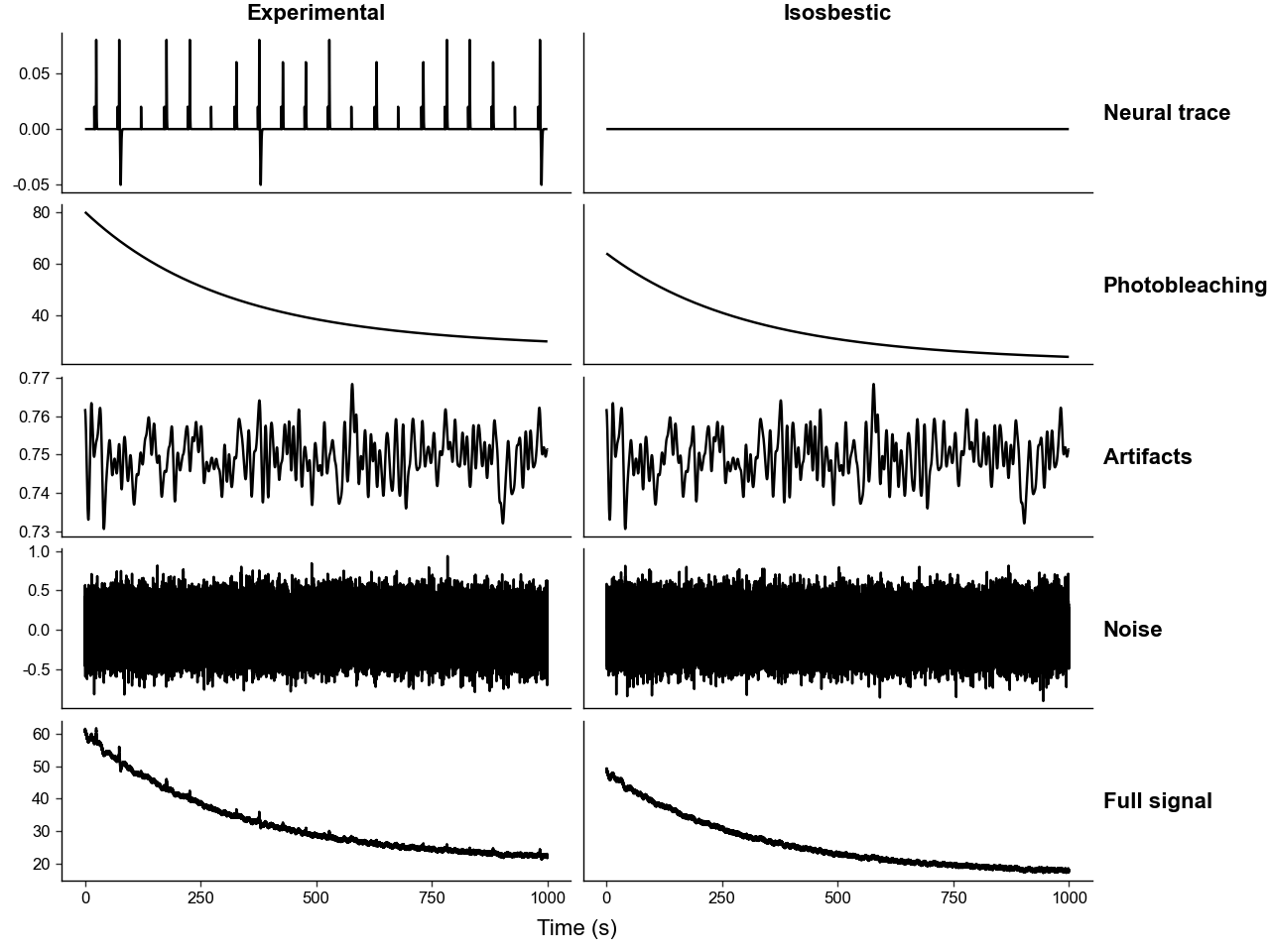
With this background knowledge, we can breakdown photometry traces into its requisite components:
- Neural trace, the "true signal"
- The changes in \(F(\lambda_{exp})\) representing the fluctuations \([L]\).
- Photobleaching attenuation
- The irreversible process of \(P_{ex} \rightarrow P_b\), decreasing overall fluorescence over time.
- Detector and electronic noise
- Guassian noise of constant magnitude over time originating from the electronic components of the detector device.
- Multiplicative noise
- Multiplicative noise whose magnitude depends on signal intensity from photonic shot-noise, laser power fluctuations, etc.
- Attenuation artifacts
- Both movement and hemodynamic artifacts that decrease the precentage of light transmitance.
- Most movement artifacts come from the bending of the fiber optic cable, which causes some light to be not be internally reflected and "lost".
- Background autofluorescence
- The fluorecent response of the tissue and fiber.
2. The Simulation Model
This package simulates photometry traces by modeling the above components of photometry traces with the following layers:
TimeBase: is used to create the time series of the traces.
-
Neural trace, the "true signal"
-
EventLayer(\(\mathbf{E}\)): fractional fluorescence changes relative to local baseline caused by changes in \([L]\) in response to input events. This can be thought of as the "true signal" we aim to recover. -
NeuralDynamicNoiseLayer(\(\mathbf{D}\)): also fractional fluorescence changes relative to local baseline caused by changes in \([L]\), but not in response to any events. This can be thought of as the "true noise" in the signal we aim to recover. Generally it is of a much lower frequency than the sampling frequency.
-
- Photobleaching attenuation & 6. background autofluorecence
PhotobleachingLayer(\(\mathbf{B}\)): models photobleaching with a negative bi-exponential equation (see below) that also captures background autofluorecence as \(\beta_{\text{floor}}\), i.e. \(\mathbf{B(t \rightarrow \infty)}\).
- Detector and electronic noise
NoiseGaussianLayer(\(\mathbf{N_g}\)): Gaussian noise of constant magnitude over time.
- Multiplicative noise
NoiseMultiplicativeLayer(\(\mathbf{N_m}\)): Noise dependent on signal intensity with \(\text{Var}(t) \propto k \cdot (I_{sig})^{p}\).
-
Attenuation artifacts
-
MovementAttenuationLayer(\(\mathbf{M}\)): low-frequency movement attenuation representing baseline movement, generated by low-pass filtering gaussian noise. -
ArtifactSpikeLayer(\(\mathbf{AS}\)): sharp pings that readily return to baseline, that represent sharp bends in the fiber optic cable, which have been observed in real data. -
ArtifactJumpLayer(\(\mathbf{AJ}\)): sharp changes in the baseline value of signal for an extended period, which have been observed in real data. -
All serve as a multiplicative mask on fluorecence, i.e. they are \(\ge 0\) and centered on \(1\).
-
Then the experimental trace is calculated by:
-
\(\text{Clean Trace} \, (\mathbf{C}) = (\mathbf{B} - \mathbf{B_{t\rightarrow \infty}}) \cdot (\mathbf{E} + \mathbf{D}) + \mathbf{B}\)
-
\(\text{Artifact} \, (\mathbf{A}) = \mathbf{M} \cdot \mathbf{AS} \cdot \mathbf{AJ}\)
-
\(\text{Noise} \, (\mathbf{N}) = \mathbf{N_g} + \mathbf{N_m}(\mathbf{C \cdot A})\)
-
\(F(\lambda_{exp}) = \mathbf{C} \cdot \mathbf{A} + \mathbf{N}\)
And the isosbestic trace is calculated by:
-
\(\text{Clean Trace} \, (\mathbf{C_{iso}}) = (\mathbf{B_{iso}} - \mathbf{B_{iso,t\rightarrow \infty}}) \cdot \text{c}_{\text{iso-leakage}} (\mathbf{E} + \mathbf{D}) + \mathbf{B_{iso}}\)
-
\(\text{Artifact} \, (\mathbf{A}) = \mathbf{M} \cdot \mathbf{AS} \cdot \mathbf{AJ}\)
-
\(\text{Noise} \, (\mathbf{N_{iso}}) = \mathbf{N_{g,iso}} + \mathbf{N_{m,iso}}(\mathbf{C_{iso} \cdot A})\)
-
\(F(\lambda_{iso}) = \mathbf{C_{iso}} \cdot \mathbf{A} + \mathbf{N_{iso}}\)
Where \(\mathbf{B}\) and \(\mathbf{N}\) are calculated seperately from the experimental trace and \(\mathbf{A}\) is shared between experimental and isosbestic traces.
Note that \((\mathbf{E} + \mathbf{D})\) is scaled by \((\mathbf{B} - \mathbf{B_{t\rightarrow \infty}})\) not just \(\mathbf{B}\). This is because the simulation assumes that the source of background fluorecence is not the target fluorophore. With this scaling term it assumes that as \(t \rightarrow \infty\), the concentration of unbleached fluorophore \(\rightarrow 0\) and, thus \((\mathbf{E} + \mathbf{D}) \rightarrow 0\).
While the ideal isosbestic wavelength will not contain any neural trace, this package supports simulating a non-ideal isosbestic wavelength with the parameter iso_event_leakage which controls how much the "true signal" leaks into the isosbestic trace. It is \(\propto \phi_{PL} \cdot \epsilon_{PL} - \phi_{P} \cdot \epsilon_P\) at the isosobestic wavelength.
If iso_event_leakage == 0, the isosbestic wavelength is "ideal" and \(F(\lambda_{iso})\) is \([L]\) agnostic. Ifiso_event_leakage > 0, the bound protein is "brighter" than the unbound protein at \(\lambda_{iso}\) and a positive change in \([L]\), and thus \(F(\lambda_{exp})\), causes a positive transient in \(F(\lambda_{iso})\). Likewise, if iso_event_leakage < 0, a positive change in \([L]\) causes a negative transient in \(F(\lambda_{iso})\).
3. Simulating Photometry
In this package, we can simulate photometry using the SimulatedPhotometry class.
SimulatedPhotometry can either be built directly from the layers in PhoPro.sim.layers or, most conviently, from parameters using .from_parameters().
# import important packages
import numpy as np
import pandas as pd
from plotnine import * # type: ignore

from PhoPro import SimulatedPhotometry
sim = SimulatedPhotometry.from_parameters(
    # length of experiment and sampling rate
    length_sec=1000,
    frequency=100,

    # parameters of photobleaching curves
    bleaching_params_exp = { 'alpha1': 50, 'alpha2': 20, 'tau1': 300, 'tau2': 10000, 'B_floor': 10 },
    bleaching_params_iso = { 'alpha1': 45, 'alpha2': 18, 'tau1': 300, 'tau2': 10000, 'B_floor': 8 },

    # you can alternatively make the photobleaching curve
    #   of the isosbestic by scaling that of the experimental
    iso_bleach_scale=None,

    # optional evenly spaced event of the E layer
    n_events=None,

    # magnitude and frequency of the M layer
    movement_attenuation=0.3,
    attenuation_cutoff_hz=0.1,

    # magnitude of the Nm layer
    mult_noise_magnitude_exp=1e-4,
    # when iso param is None, it default to exp value
    mult_noise_magnitude_iso=None,
    # how Nm scales with intensity
    mult_noise_exponent_exp=1.0,

    # magnitude of the Ng layer
    gaussian_noise_scale_exp=0.2,
    # when iso param is None, it default to exp value
    gaussian_noise_scale_iso=None,

    # magnitude, offset, and frequency of the D layer
    dynamic_noise_amplitude=0.001,
    dynamic_noise_center=0.0,
    dynamic_noise_frequency=1.0,

    # controls for the AS layer
    n_spike_artifacts=5,
    spike_amplitude_range=(-0.5, -0.2),

    # controls for the AJ layer
    n_jump_artifacts=2,
    jump_amplitude_range=(0.3, 0.35),
    jump_duration_range=(100, 200),

    # reproducible rng
    seed=102,

    # isosbestic leakage control
    iso_event_leakage=None,
)
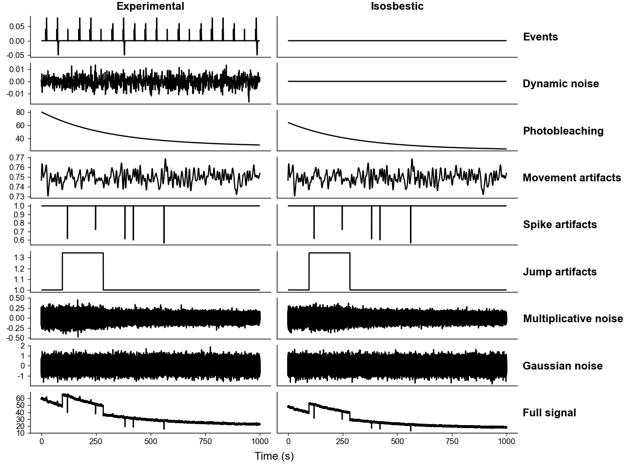
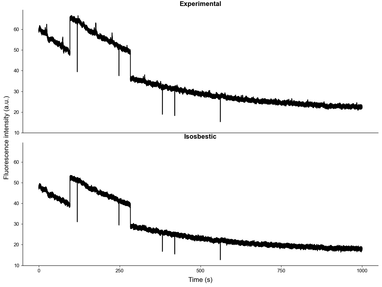
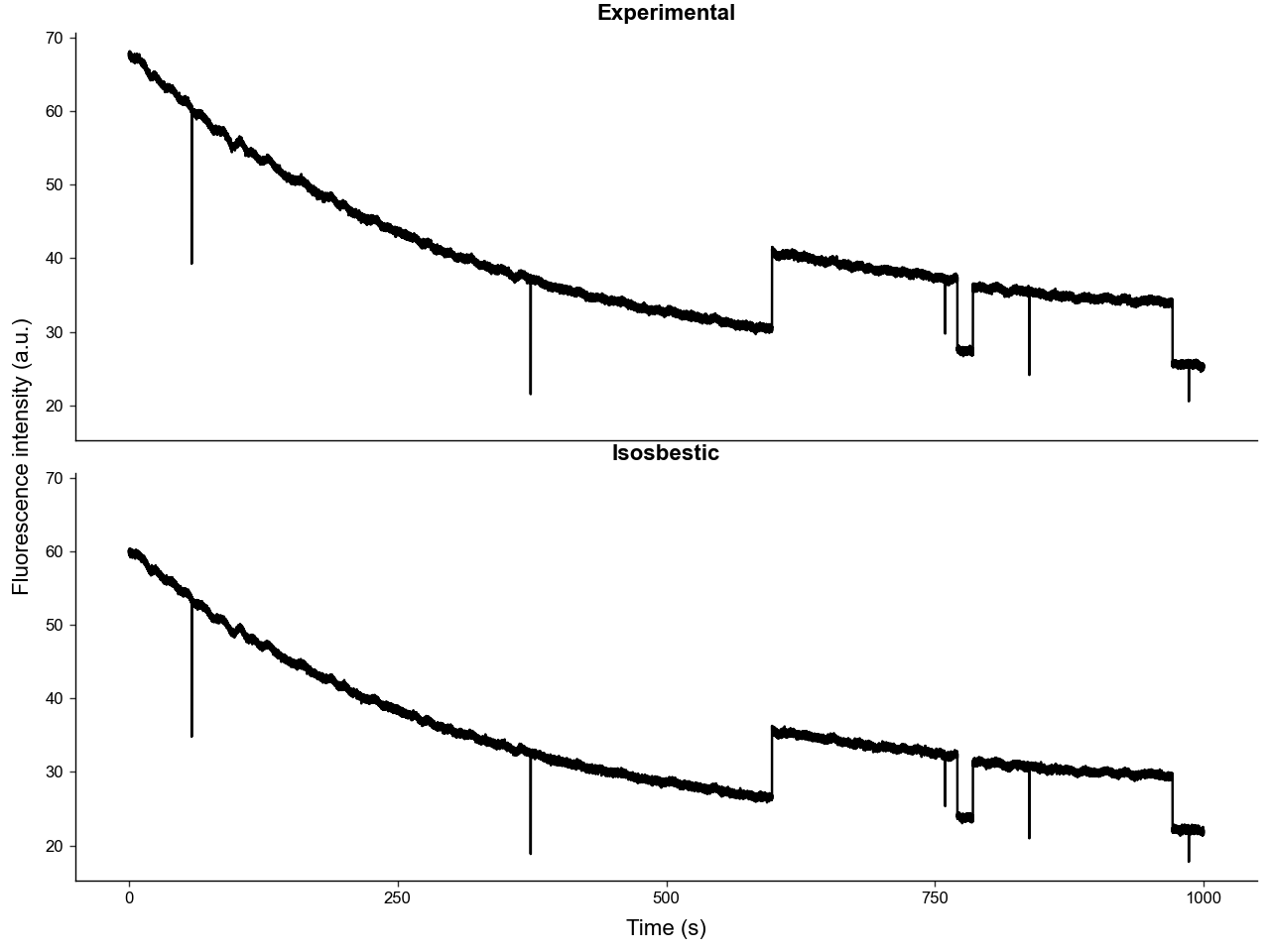
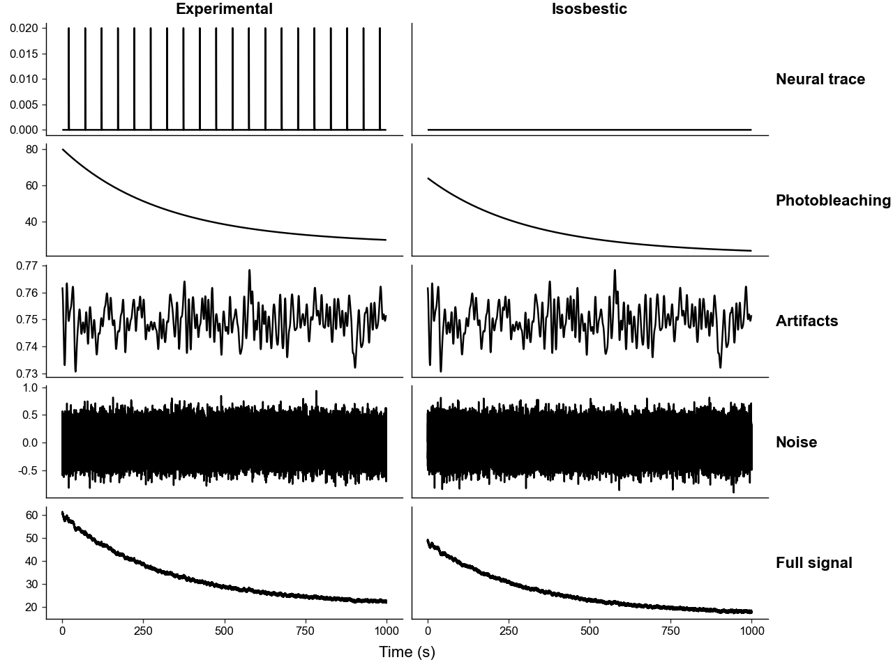
We can visualize the trace components and the final composite traces using .plot_layers() and .plot_traces().
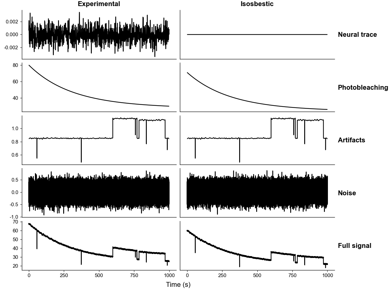
Note that you can see how the intemediate layers are constructed from the base ones by comparing the condensed and full plots.
4. Controling Event Responses
For simulated data to be useful, we need to add "true signal", i.e. neural responses to events. We can do this both during the construction of SimulatedPhotometry and after.
Each event response is based on a kernel function, which take in a time-point array, an amplitude, and any number of other parameters, and produce a shape. Many kernel functions have been provided as static methods of SimulatedPhotometry, all starting with "kernel_*".
Let's take a look at how the gamma kernel behaves.
from PhoPro.utils.graphing import get_default_theme

def plot_gamma_across_ks(shape_ks: list[float] = [2, 3, 4, 5], tau_sec: float = 1.0, amplitude: float = 1.0) -> None:
    time = np.linspace(0, 10, 1000)

    dfs: list[pd.DataFrame] = []
    for shape_k in shape_ks:
        df_i = pd.DataFrame({
            'time' : time,
            'shape_k' : str(shape_k),
            'value' : SimulatedPhotometry.kernel_gamma(time, amplitude, shape_k, tau_sec)
        })
        dfs.append(df_i)

    df = pd.concat(dfs, ignore_index=True)

    p = (
        ggplot(df, aes(x='time', y='value', color='shape_k'))
        + geom_line()
        + labs(title=f'Gamma kernel across shape_k\'s at tau_sec = {tau_sec}')
        + get_default_theme()
    )
    p.show()

def plot_gamma_across_taus(tau_secs: list[float] = [0.5, 1, 1.5], shape_k: float = 3, amplitude: float = 1.0) -> None:
    time = np.linspace(0, 10, 1000)

    dfs: list[pd.DataFrame] = []
    for tau_sec in tau_secs:
        df_i = pd.DataFrame({
            'time' : time,
            'tau_sec' : str(tau_sec),
            'value' : SimulatedPhotometry.kernel_gamma(time, amplitude, shape_k, tau_sec)
        })
        dfs.append(df_i)

    df = pd.concat(dfs, ignore_index=True)

    p = (
        ggplot(df, aes(x='time', y='value', color='tau_sec'))
        + geom_line()
        + labs(title=f'Gamma kernel across tau_sec\'s at shape_k = {shape_k}')
        + get_default_theme()
    )
    p.show()


plot_gamma_across_ks()
plot_gamma_across_taus()
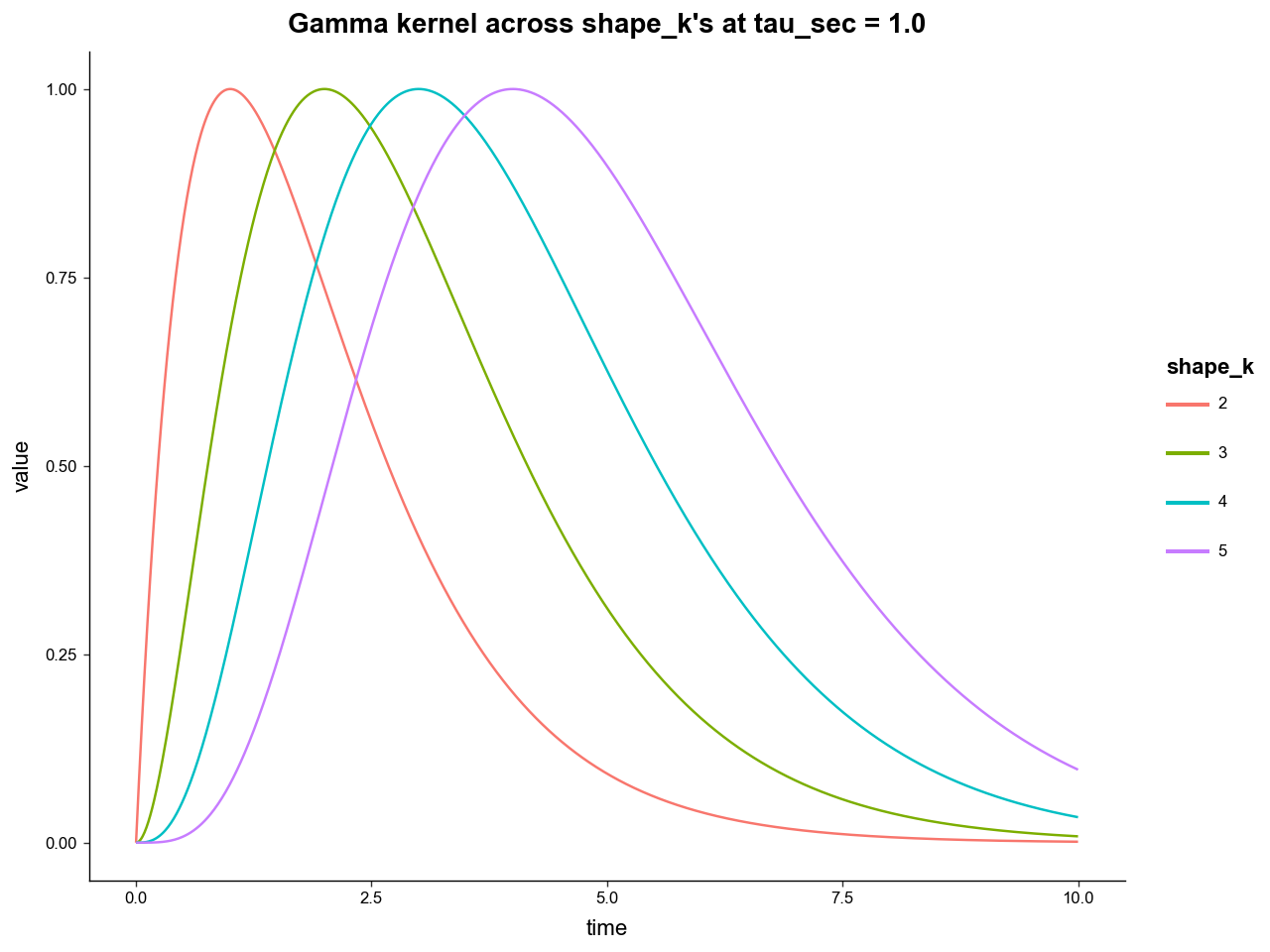
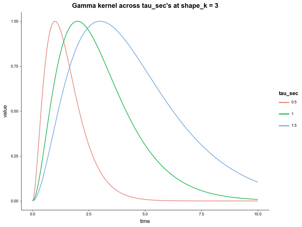
We see how the "shape_k" parameter controls the rate of increase, while the "tau_sec" parameter controls the rate of decay (roughly).
Now let's add some events to our simulated data.
sim = SimulatedPhotometry.from_parameters(
    # --- event params ---
    # evenly spaced events of the E layer
    # these are best used as the "trial_cue" event
    n_events=20,
    event_label='trial_cue',

    # how much time in seconds to leave at either end of the trace
    event_buffer_sec=20.0,

    # the kernel function to generate event response architecture
    event_kernel=SimulatedPhotometry.kernel_gamma,
    # its amplitude
    event_amplitude=0.02,
    # other params for the kernel function
    event_kernel_params={ 'shape_k' : 3 , 'tau_sec' : 0.1},

    # --- other ---
    # length of experiment and sampling rate
    length_sec=1000,
    frequency=100,

    # parameters of photobleaching curves
    bleaching_params_exp = { 'alpha1': 50, 'alpha2': 20, 'tau1': 300, 'tau2': 10000, 'B_floor': 10 },
    iso_bleach_scale=0.8,
)

# now we can see the events in the experimental neural trace layer
sim.plot_layers()
We can add more events after construction using .add_event() and .add_event_relative_to(). The latter is generally more useful for simulating experimental data since you can add events relative to a "trial_cue" event and choice lock multiple events.
Below we will add events to reconstruct the same experiment used as an example in the Introduction tutorial, wherein:
-
A light turns on signifying the beginning of trial, represented by "trial_cue".
-
Then the rat has between 2 and 4 seconds after the "trial_cue" to choose 1 of 2 levers that when pressed register as "lever1" and "lever2".
-
"lever1" gives the rat a large food reward but there is a chance of the rat being shocked immediately after, represented by the "shock" event.
-
"lever2" gives the rat a small food reward.
# add lever press events
sim.add_event_relative_to(

    relative_to='trial_cue',

    # time range after "relative_to" onset the new events can be placed
    time_range=(2, 4),

    # the overall probability of any event happening
    overall_prob=0.8,

    # event specifications
    labels=['lever1', 'lever2'],
    amplitudes=[0.08, 0.06],
    kernel_funcs=[
        SimulatedPhotometry.kernel_gamma,
        SimulatedPhotometry.kernel_gamma
    ],
    kernel_params=[
        {'shape_k':5, 'tau_sec':0.2},
        {'shape_k':5, 'tau_sec':0.2},
    ],

    # the relative probabilties of the events
    choice_probs=[0.5, 0.5],
)

sim.add_event_relative_to(
    relative_to='lever1',
    time_range=(1, 1.5),
    overall_prob=0.5,
    labels=['shock'],
    amplitudes=[-0.05],
    kernel_funcs=[
        SimulatedPhotometry.kernel_gamma
    ],
    kernel_params=[
        {'shape_k':10, 'tau_sec':0.3},
    ],
)

# now we can see all the events in the experimental neural trace layer
sim.plot_layers()
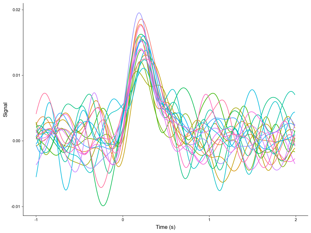
5. Using Simulated Data
The main utility of simulating data is to allow for comparsions between processing methods with the ground truth of the neural signal known. The traces from SimulatedPhotometry can be directly exported to PhotometryExperiment, while the true neural signal can be directly exported to PhotometryData. After performing preprocessing and trial extraction on the PhotometryExperiment object, the resulting recovered signal in .trial_data can be compared to the exported true signal after normalization.
# similar simulated data as above
sim = SimulatedPhotometry.from_parameters(
    length_sec=1000,
    frequency=100,
    bleaching_params_exp = { 'alpha1': 50, 'alpha2': 20, 'tau1': 300, 'tau2': 10000, 'B_floor': 10 },
    iso_bleach_scale=0.8,

    n_events=20,
    event_label='trial_cue',
    event_buffer_sec=20.0,

    event_kernel=SimulatedPhotometry.kernel_gamma,
    event_amplitude=0.02,
    event_kernel_params={ 'shape_k' : 3 , 'tau_sec' : 0.1},
)
# export to Photometry experiment, process, and window
exp = sim.to_PhotometryExperiment()

exp.preprocess_signal(
    correction_method='dF/F',
    fit_using='IRLS'
)

exp.extract_trial_data(
    align_to='trial_cue',
    trial_bounds=(-1, 2),
)

recovered_signal = exp.trial_data

# get true signal, ensure that extraction parameters are the same
true_signal = sim.to_PhotometryData(
    align_to='trial_cue',
    trial_bounds=(-1, 2)
)
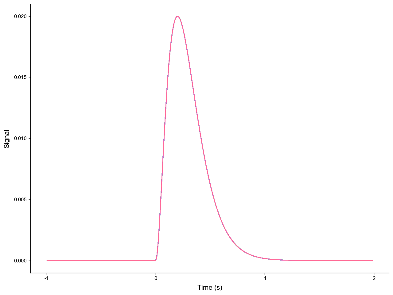
Now lets compute some metrics on how well we recovered the true signal.
# since all true signals are the same we can collapse them
# then we will get the signals as arrays from the .X attribute
true_arr = true_signal.collapse(None).X
recoved_arr = recovered_signal.X

# compute error metrics
err = recoved_arr - true_arr
rmsd = np.sqrt(np.mean(err**2, axis=1))
mae = np.mean(np.abs(err), axis=1)

# add them as columns in .obs
recovered_signal.obs['rmsd'] = rmsd
recovered_signal.obs['mae'] = mae

# print error information
print(
    f'RMSD = {np.mean(rmsd):.4f} +/- {np.std(rmsd):.4f}\n'
    f'MAE = {np.mean(mae):.4f} +/- {np.std(mae):.4f}'
)
RMSD = 0.0030 +/- 0.0008
MAE = 0.0024 +/- 0.0006
By comparing the error metrics of multiple different preprocessing methods we can better understand what methods are most accurate for different types of real-world data.
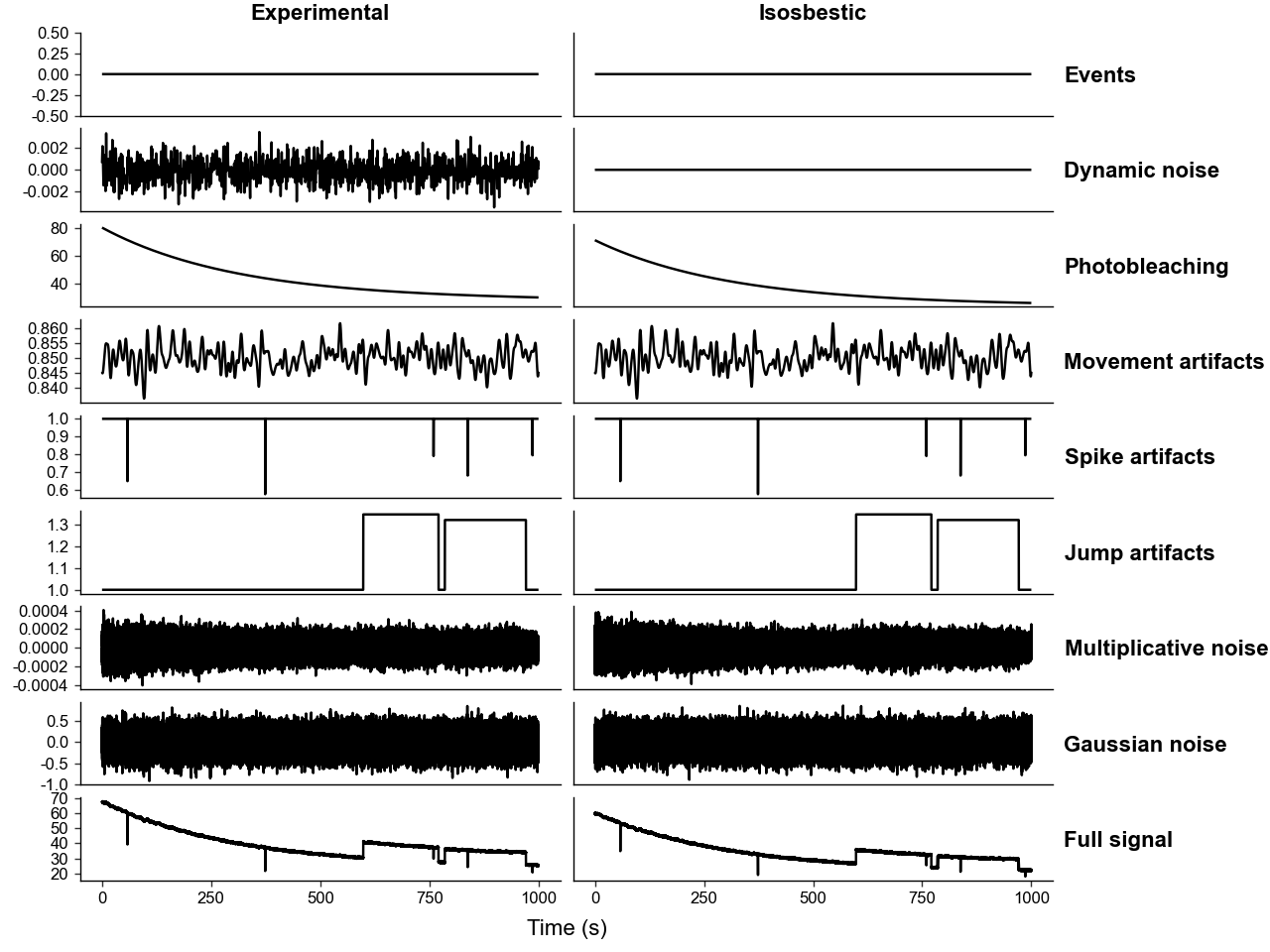
6. A peek behind the curtain
The example data used in the Introduction tutorial was generated by the code below:
sim = SimulatedPhotometry.from_parameters(
    length_sec=1000,
    frequency=100,

    bleaching_params_exp = { 'alpha1': 50, 'alpha2': 20, 'tau1': 300, 'tau2': 10000, 'B_floor': 10 },
    iso_bleach_scale=0.8,
    iso_bleach_offset=None,

    event_label='trial_cue',
    n_events=20,
    event_kernel=SimulatedPhotometry.kernel_gamma,
    event_amplitude=0.04,
    event_kernel_params={'tau_sec':0.1},
    event_buffer_sec=20.0,

    movement_attenuation=0.5,
    attenuation_cutoff_hz=0.1,

    mult_noise_magnitude_exp=0.1,
    gaussian_noise_scale_exp=0.4,

    dynamic_noise_amplitude=0.004,
    dynamic_noise_center=0.0,
    dynamic_noise_frequency=1.0,

    n_spike_artifacts=5,
    spike_amplitude_range=(-0.5, -0.2),

    n_jump_artifacts=1,
    jump_amplitude_range=(0.3, 0.35),
    jump_duration_range=(100, 200),

)

sim.add_event_relative_to(
    relative_to='trial_cue',
    time_range=(2, 4),
    overall_prob=0.8,
    labels=['lever1', 'lever2'],
    choice_probs=[0.5, 0.5],
    amplitudes=[0.08, 0.06],
    kernel_funcs=[
        SimulatedPhotometry.kernel_gamma,
        SimulatedPhotometry.kernel_gamma
    ],
    kernel_params=[
        {'shape_k':5, 'tau_sec':0.2},
        {'shape_k':5, 'tau_sec':0.2},
    ],
)

sim.add_event_relative_to(
    relative_to='lever1',
    time_range=(1, 1.5),
    overall_prob=0.5,
    labels=['shock'],
    amplitudes=[-0.05],
    kernel_funcs=[
        SimulatedPhotometry.kernel_gamma
    ],
    kernel_params=[
        {'shape_k':10, 'tau_sec':0.3},
    ],
)

sim.plot_layers(condensed=False).show()
sim.plot_traces().show()