Signal Processing
This tutorial gives an in depth overview of the PhotometryExperiment class. PhotometryExperiment represents one continuous photometry recording and provides tools for preprocessing traces, inspecting reference fits, trimming recordings, exporting continuous data, and extracting trial-wise PhotometryData.
The most important idea is that PhotometryExperiment works with continuous data, while PhotometryData works with trial-wise data.
A typical workflow is:
-
Load a continuous experiment.
-
Inspect raw traces and event labels.
-
Preprocess the continuous signal.
-
Extract trial windows around behavioral events.
-
Analyze or save the resulting
PhotometryDataobject.
Setup
First we import the packages used throughout the tutorial.
import numpy as np
import pandas as pd
from plotnine import * # type: ignore

from PhoPro import PhotometryExperiment, PhotometryData
The examples below use the bundled CSV experiment. To keep each section independent, we will define helper functions that reload a fresh experiment whenever needed.
EVENT_COLS = ['trial_cue', 'lever1', 'lever2', 'shock']


def load_example(isosbestic: bool = True) -> PhotometryExperiment:
    return PhotometryExperiment.load_CSV(
        csv='data/experiments/example_experiment.csv',
        time_col='time',
        signal_col='raw_signal',
        isosbestic_col='raw_isosbestic' if isosbestic else None,
        event_cols=EVENT_COLS,
        annotation_file='data/experiments/example_annotation.json',
        annotation_handler='json',
    )


def load_processed(**preprocess_kwargs) -> PhotometryExperiment:
    exp = load_example()
    exp.id = 'Processed example'
    kwargs = dict(
        cutoff_frequency=3,
        order=4,
        correction_method='dF/F',
        fit_using='IRLS',
        maxiter=2000,
        c=2,
    )
    kwargs.update(preprocess_kwargs)
    exp.preprocess_signal(**kwargs)
    return exp
1. Loading a Continuous Experiment
PhotometryExperiment can be created directly from arrays, but most workflows use a loader. The convenience class methods load_CSV and load_TDT create the appropriate loader and return a PhotometryExperiment.
Dual channel photometry experiment with 100000 timepoints.
A dual-channel experiment contains both the experimental signal and an isosbestic reference. A single-channel experiment has only the experimental signal.
dual
True
100000
99.90109791306607
The continuous arrays are stored on the object. time aligns with raw_signal and, when present, raw_isosbestic.
[0.   0.01 0.02 0.03 0.04]
[60.72501182 59.62409786 60.76089457 60.44649406 59.42376882]
[48.43589551 47.4642179  46.94416148 48.21042178 47.25050209]
Events are stored in a dictionary mapping event labels to timestamp arrays.
['trial_cue', 'lever1', 'lever2', 'shock']


{'trial_cue': 20, 'lever1': 9, 'lever2': 6, 'shock': 3}
Metadata from annotation files is stored in metadata. Built-in loaders also include the source file path.
{'source': 'data/experiments/example_experiment.csv',
 'subject': 'animal_1',
 'sex': 'male',
 'age': 'young'}
2. Inspecting Raw Data
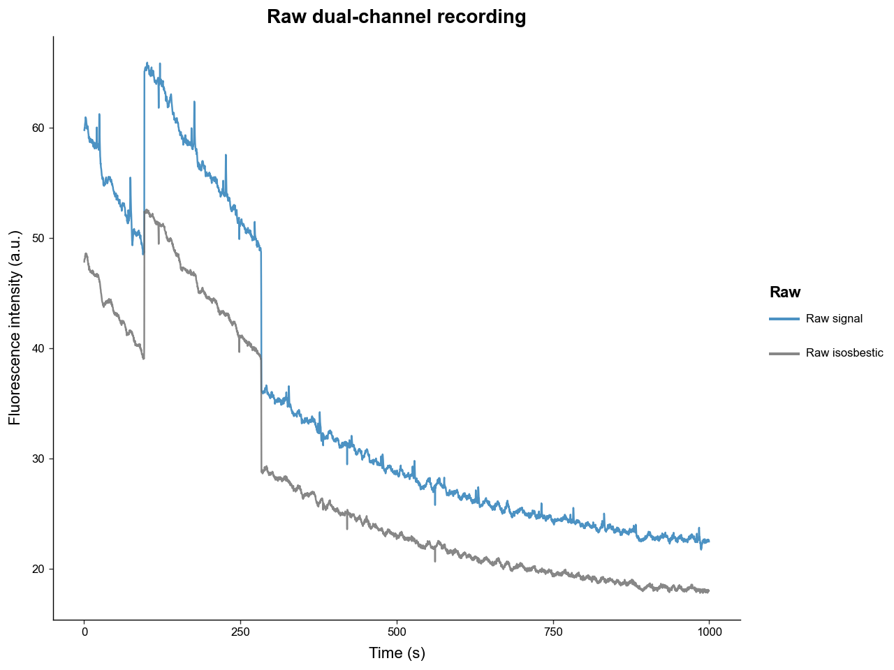
plot_dashboard gives a quick view of the continuous recording. Before preprocessing, raw='auto' shows the raw signal and raw isosbestic traces.
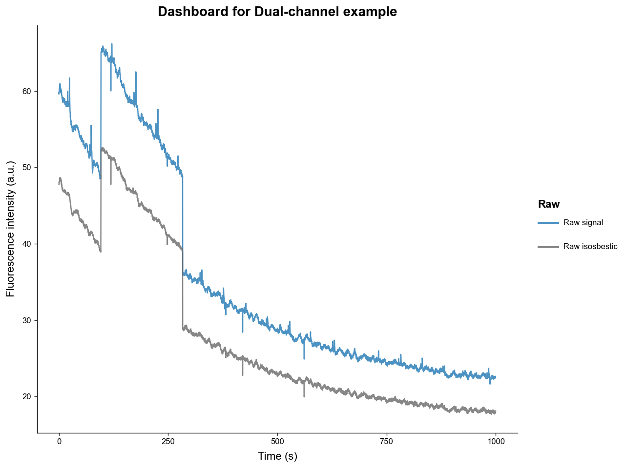
The plotting methods return plotnine objects, so they can be modified before display.
Continuous data can also be inspected as a dataframe. to_wide_dataframe keeps one row per timepoint.
| time | raw_signal | raw_isosbestic | trial_cue | lever1 | lever2 | shock | |
|---|---|---|---|---|---|---|---|
| 0 | 0.495 | 59.842783 | 47.942846 | False | False | False | False |
| 1 | 1.495 | 60.270320 | 48.244646 | False | False | False | False |
| 2 | 2.495 | 60.875302 | 48.473810 | False | False | False | False |
| 3 | 3.495 | 60.532914 | 48.501635 | False | False | False | False |
| 4 | 4.495 | 59.995382 | 48.312218 | False | False | False | False |
to_long_dataframe keeps one row per timepoint and trace source. This is the format used by the dashboard plotting helper.
| time | source | value | |
|---|---|---|---|
| 0 | 0.495 | raw_signal | 59.842783 |
| 1 | 1.495 | raw_signal | 60.270320 |
| 2 | 2.495 | raw_signal | 60.875302 |
| 3 | 3.495 | raw_signal | 60.532914 |
| 4 | 4.495 | raw_signal | 59.995382 |
3. Low-pass Filtering and Reference Fitting
preprocess_signal combines the main preprocessing steps, but the lower-level helpers are also available. The first step is usually a low-pass Butterworth filter.
filtered_signal = exp.low_frequency_pass_butter(
    signal=exp.raw_signal,
    sample_frequency=exp.frequency,
    cutoff_frequency=3,
    order=4,
)

filtered_isosbestic = exp.low_frequency_pass_butter(
    signal=exp.raw_isosbestic,
    sample_frequency=exp.frequency,
    cutoff_frequency=3,
    order=4,
)

filtered_signal[:5]
array([60.71852848, 60.60089085, 60.48557731, 60.37416651, 60.26810553])
In dual-channel experiments, the isosbestic trace is fitted to the experimental signal before correction. The package supports ordinary least squares and iteratively reweighted least squares, with or without an intercept.
fitted_ref, r2_val, coeffs = exp.fit_isosbestic_to_signal(
    signal=filtered_signal,
    isosbestic=filtered_isosbestic,
    fit_using='IRLS',
    maxiter=2000,
    c=2,
)

print(r2_val)
print(coeffs)
0.9993291237999945
[-0.00914491  1.25010411]
The fitted reference is the trace that will be subtracted or divided away during preprocessing.
pd.DataFrame({
    'time': exp.time[:5],
    'filtered_signal': filtered_signal[:5],
    'filtered_isosbestic': filtered_isosbestic[:5],
    'fitted_reference': fitted_ref[:5],
})
| time | filtered_signal | filtered_isosbestic | fitted_reference | |
|---|---|---|---|---|
| 0 | 0.00 | 60.718528 | 48.483138 | 60.599827 |
| 1 | 0.01 | 60.600891 | 48.388588 | 60.481628 |
| 2 | 0.02 | 60.485577 | 48.293900 | 60.363258 |
| 3 | 0.03 | 60.374167 | 48.200785 | 60.246857 |
| 4 | 0.04 | 60.268106 | 48.110847 | 60.134422 |
4. Dual-channel Preprocessing
preprocess_signal runs filtering, reference fitting, correction, optional whole-signal normalization, and optional artifact correction. For many dual-channel experiments, a 3 Hz low-pass filter, IRLS reference fitting, and dF/F correction are a reasonable starting point.
exp = load_processed()

print(exp.has_ran_preprocess)
print(exp.signal.shape)
print(exp.fitted_ref.shape)
True
(100000,)
(100000,)
After preprocessing, several attributes are populated:
-
filt_sig: filtered experimental signal. -
filt_iso: filtered isosbestic signal for dual-channel data. -
fitted_ref: fitted reference trace. -
signal: final processed signal. -
metadata['reference_fit']: fit type, fit quality, and coefficients. -
metadata['correction_method']: the correction method used.
{'type': 'isosbestic',
 'r2_val': 0.9993291237999945,
 'coeffs': array([-0.00914491,  1.25010411])}
'dF/F'
After preprocessing, plot_dashboard(raw=False) shows the filtered signal, fitted reference, and processed trace.
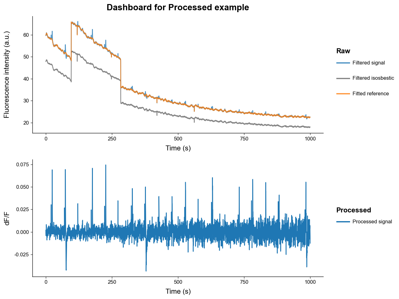
The correction method can be changed. dF/F returns (signal - fitted_reference) / fitted_reference. dF returns signal - fitted_reference.
df_exp = load_processed(correction_method='dF')

print(df_exp.metadata['correction_method'])
print(df_exp.signal[:5])
dF
[0.11870166 0.11926243 0.12231895 0.12730982 0.13368323]
Whole-signal normalization can be applied after correction. Built-in options are 'none', 'zscore', and 'nullZ'.
z_exp = load_processed(signal_normalization='zscore')

print(np.mean(z_exp.signal))
print(np.std(z_exp.signal))
7.958078640513121e-18
1.0
Custom correction and normalization functions can be passed directly. A custom correction function receives signal and fitted_ref and must return a one-dimensional processed signal.
def percent_dF_F(signal: np.ndarray, fitted_ref: np.ndarray) -> np.ndarray:
    return 100 * (signal - fitted_ref) / np.maximum(fitted_ref, np.finfo(np.float32).eps)

custom_exp = load_processed(correction_method=percent_dF_F)

print(custom_exp.metadata['correction_method'])
print(custom_exp.signal[:5])
percent_dF_F
[0.19587789 0.19718786 0.20263808 0.21131362 0.22230733]
5. Single-channel Preprocessing
Single-channel experiments do not have an isosbestic reference. In that case, preprocess_signal fits a photobleaching curve and uses single-channel correction methods such as dB/B or dB.
single
False
single.preprocess_signal(
    cutoff_frequency=3,
    order=4,
    correction_method='dB/B',
    signal_normalization='none',
    channel_mode='single',
)

print(single.metadata['reference_fit']['type'])
print(single.metadata['reference_fit']['r2_val'])
photobleaching
0.8032179060068196
The photobleaching curve can also be fit directly with fit_photobleaching_curve.
bleach_curve, bleach_r2, bleach_params = single.fit_photobleaching_curve(
    signal=single.filt_sig,
)

print(bleach_r2)
print(bleach_params)
0.8032179060068196
[5.38883450e-10 5.00005000e-03 4.00708720e+01 3.11392112e-03
 2.05621528e+01]
6. Optional Artifact Detection and Correction
preprocess_signal accepts an artifact_detector and artifact_corrector. Detectors identify artifact intervals and correctors replace or adjust the processed signal in those intervals.
Artifact settings are experiment-specific, so the safest pattern is to inspect the raw and processed traces, tune the detector on representative recordings, then apply the chosen detector and corrector consistently.
from PhoPro.analysis.artifact import ODS_Detector, Spline_Corrector

# Example configuration. Tune thresholds for your own data before using it in production.
detector = ODS_Detector(
    score_threshold=8,
    jump_score_threshold=8,
    expand_sec=(0.5, 2),
    buffer_sec=1.5,
    n_chunks=50,
)

corrector = Spline_Corrector(
    anchor_sec=(0.2, 0.2),
    correct_spikes=True,
    correct_jumps=True,
)

print(detector)
print(corrector)
<PhoPro.analysis.artifact.ODS_Detector object at 0x3279dfa90>
<PhoPro.analysis.artifact.Spline_Corrector object at 0x3216bb890>
To run artifact correction, pass the detector and corrector to preprocess_signal. This cell is commented out so the tutorial does not imply that one detector configuration is universally appropriate.
# artifact_exp = load_example()
# artifact_exp.preprocess_signal(
#     cutoff_frequency=3,
#     order=4,
#     correction_method='dF/F',
#     fit_using='IRLS',
#     artifact_detector=detector,
#     artifact_corrector=corrector,
# )
# artifact_exp.artifacts.df.head()
7. Trimming Continuous Recordings
trim_times_by_index and trim_times_by_values remove timepoints from the continuous recording. They also trim every present trace and remove event timestamps outside the new time range.
It is best to trim before trial extraction or artifact correction so all derived results stay aligned.
trimmed = load_example()
trimmed.trim_times_by_values(lower=100, upper=200)

print(trimmed.time[0], trimmed.time[-1])
print(trimmed.n_times)
print({k: len(v) for k, v in trimmed.events.items()})
100.0 200.0
10001
{'trial_cue': 2, 'lever1': 1, 'lever2': 0, 'shock': 0}
Index trimming uses an inclusive start_idx and an exclusive stop_idx.
trimmed_by_index = load_example()
trimmed_by_index.trim_times_by_index(start_idx=1000, stop_idx=2000)

print(trimmed_by_index.time[0], trimmed_by_index.time[-1])
print(trimmed_by_index.raw_signal.shape)
10.0 19.99
(1000,)
8. Exporting Continuous Data
Continuous experiment traces can be exported as wide or long dataframes. The export methods include whatever traces are available at the time they are called.
| time | raw_signal | raw_isosbestic | processed_signal | fitted_reference | filtered_signal | filtered_isosbestic | trial_cue | lever1 | lever2 | shock | |
|---|---|---|---|---|---|---|---|---|---|---|---|
| 0 | 0.495 | 59.842783 | 47.942846 | -0.001494 | 59.955814 | 59.865875 | 47.967974 | False | False | False | False |
| 1 | 1.495 | 60.270320 | 48.244646 | -0.000418 | 60.297531 | 60.272064 | 48.241322 | False | False | False | False |
| 2 | 2.495 | 60.875302 | 48.473810 | 0.004628 | 60.604191 | 60.884103 | 48.486630 | False | False | False | False |
| 3 | 3.495 | 60.532914 | 48.501635 | -0.001277 | 60.611847 | 60.534332 | 48.492754 | False | False | False | False |
| 4 | 4.495 | 59.995382 | 48.312218 | -0.006628 | 60.393551 | 59.993045 | 48.318133 | False | False | False | False |
| time | source | value | |
|---|---|---|---|
| 0 | 0.495 | raw_signal | 59.842783 |
| 1 | 1.495 | raw_signal | 60.270320 |
| 2 | 2.495 | raw_signal | 60.875302 |
| 3 | 3.495 | raw_signal | 60.532914 |
| 4 | 4.495 | raw_signal | 59.995382 |
Use write_csv when you want to save the continuous traces to disk.
exp.write_csv(
    file='output/processed_experiment_wide.csv',
    downsample=100,
    export_events=True,
    format='wide',
)

pd.read_csv('output/processed_experiment_wide.csv').head()
| Unnamed: 0 | time | raw_signal | raw_isosbestic | processed_signal | fitted_reference | filtered_signal | filtered_isosbestic | trial_cue | lever1 | lever2 | shock | |
|---|---|---|---|---|---|---|---|---|---|---|---|---|
| 0 | 0 | 0.495 | 59.842783 | 47.942846 | -0.001494 | 59.955814 | 59.865875 | 47.967974 | False | False | False | False |
| 1 | 1 | 1.495 | 60.270320 | 48.244646 | -0.000418 | 60.297530 | 60.272064 | 48.241322 | False | False | False | False |
| 2 | 2 | 2.495 | 60.875302 | 48.473810 | 0.004628 | 60.604190 | 60.884103 | 48.486630 | False | False | False | False |
| 3 | 3 | 3.495 | 60.532914 | 48.501635 | -0.001277 | 60.611847 | 60.534332 | 48.492754 | False | False | False | False |
| 4 | 4 | 4.495 | 59.995382 | 48.312218 | -0.006628 | 60.393550 | 59.993045 | 48.318133 | False | False | False | False |
9. Extracting Trial Data
After preprocessing, extract_trial_data slices the continuous signal into trial windows and stores the result in trial_data as a PhotometryData object.
The key arguments are:
-
align_to: event label, event labels, timestamp, or timestamps that define candidate trials. -
center_on: optional event label or labels used as time zero inside each trial. -
trial_bounds: window bounds relative to the final trial center. -
event_tolerences: event annotation windows relative to the originalalign_totimestamp. -
baseline_bounds: optional baseline window bounds relative toalign_to. -
trial_normalization: optional per-trial normalization using the baseline window. -
window_alignment:'nearest'sampled windows or'interp'exact interpolated grids. -
invalid_window_policy:'drop'or'error'for windows outside the recording.
trial_exp = load_processed()

trial_exp.extract_trial_data(
    align_to='trial_cue',
    center_on=['lever1', 'lever2'],
    trial_bounds=(-8, 8),
    event_tolerences={
        'lever1': (2, 4),
        'lever2': (2, 4),
        'shock': None,
    },
    baseline_bounds=(-5, -1),
    trial_normalization='zscore',
    check_overlap=True,
    all_events=True,
    window_alignment='nearest',
)

trials = trial_exp.trial_data
trials
Photometry dataset with 20 trials, 1598 timepoints, and 5 observations.
The extracted trials are now avaliable a an PhotometryData object as the trial_data attribute.
| trial_num | trial_cue | lever1 | lever2 | shock | |
|---|---|---|---|---|---|
| 0 | 1 | -3.52 | 0.0 | NaN | NaN |
| 1 | 2 | -2.71 | 0.0 | NaN | 1.22 |
| 2 | 3 | 0.00 | NaN | NaN | NaN |
| 3 | 4 | -3.94 | 0.0 | NaN | NaN |
| 4 | 5 | -3.79 | 0.0 | NaN | NaN |
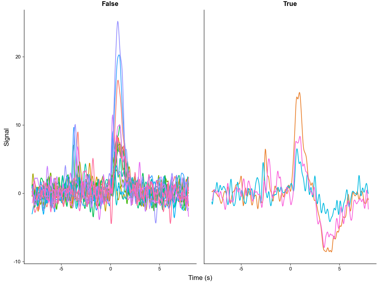
p = (
    trials
    .mutate_obs(
        has_shock = lambda d: ~d.obs['shock'].isna(),
    )
    .plot_trials(
        group_on='has_shock',
        downsample=4,
    )
)

p.show()
If baseline_bounds is supplied, the baseline windows are stored separately as baseline_data.
Photometry dataset with 20 trials, 400 timepoints, and 4 observations.
10. Alignment and Centering Semantics
align_to defines which candidate timestamps become trials. center_on decides where time zero should be in each extracted trial.
If no selected center_on event is present for a trial, that trial remains centered on its align_to timestamp.
cue_centered = load_processed()
cue_centered.extract_trial_data(
    align_to='trial_cue',
    center_on=None,
    trial_bounds=(-4, 6),
    trial_normalization='none',
)

cue_centered.trial_data.obs.head()
| trial_num | trial_cue | lever1 | lever2 | shock | |
|---|---|---|---|---|---|
| 0 | 1 | 0.0 | 3.52 | NaN | NaN |
| 1 | 2 | 0.0 | 2.71 | NaN | 3.93 |
| 2 | 3 | 0.0 | NaN | NaN | NaN |
| 3 | 4 | 0.0 | 3.94 | NaN | NaN |
| 4 | 5 | 0.0 | 3.79 | NaN | NaN |
align_to can also receive multiple labels. In that case, all timestamps are pooled and an align_event column records which event created each trial.
choice_aligned = load_processed()
choice_aligned.extract_trial_data(
    align_to=['lever1', 'lever2'],
    center_on=None,
    trial_bounds=(-4, 4),
    event_tolerences={'shock': (-1, 2)},
    trial_normalization='none',
    invalid_window_policy='drop',
)

choice_aligned.trial_data.obs.head()
| trial_num | align_event | ALIGNMENTS | shock | trial_cue | lever1 | lever2 | |
|---|---|---|---|---|---|---|---|
| 0 | 1 | lever1 | 0.0 | NaN | -3.52 | 0.0 | NaN |
| 1 | 2 | lever1 | 0.0 | 1.22 | -2.71 | 0.0 | NaN |
| 2 | 3 | lever1 | 0.0 | NaN | -3.94 | 0.0 | NaN |
| 3 | 4 | lever1 | 0.0 | NaN | -3.79 | 0.0 | NaN |
| 4 | 5 | lever2 | 0.0 | NaN | -3.56 | NaN | 0.0 |
Numeric timestamps are accepted too, which is useful for manually defined windows or external event tables.
manual_aligned = load_processed()
manual_aligned.extract_trial_data(
    align_to=[100.0, 200.0, 300.0],
    center_on=None,
    trial_bounds=(-2, 2),
    trial_normalization='none',
)

manual_aligned.trial_data.obs.head()
| trial_num | ALIGNMENTS | trial_cue | lever1 | lever2 | shock | |
|---|---|---|---|---|---|---|
| 0 | 1 | 0.0 | NaN | NaN | NaN | NaN |
| 1 | 2 | 0.0 | NaN | NaN | NaN | NaN |
| 2 | 3 | 0.0 | NaN | NaN | NaN | NaN |
11. Window Alignment: Nearest vs Interp
window_alignment='nearest' rounds each requested window to sampled timepoints. window_alignment='interp' interpolates the signal onto an exact centered grid. Both return fixed-size trial matrices, but the time grids can differ slightly.
nearest_exp = load_processed()
nearest_exp.extract_trial_data(
    align_to='trial_cue',
    center_on='lever1',
    trial_bounds=(-2, 4),
    trial_normalization='none',
    window_alignment='nearest',
)

interp_exp = load_processed()
interp_exp.extract_trial_data(
    align_to='trial_cue',
    center_on='lever1',
    trial_bounds=(-2, 4),
    trial_normalization='none',
    window_alignment='interp',
)

print(nearest_exp.trial_data.ts[:5])
print(interp_exp.trial_data.ts[:5])
[-2.00198   -1.9919701 -1.9819602 -1.9719503 -1.9619404]
[-2.        -1.9899901 -1.9799802 -1.9699703 -1.9599604]
12. Invalid Windows
A trial window is invalid if the requested trial or baseline interval extends outside the continuous recording. invalid_window_policy='error' makes this explicit. 'drop' removes those trials and records their indexes in metadata['invalid_windows'].
edge_case = load_processed()

try:
    edge_case.extract_trial_data(
        align_to=[1.0, 100.0],
        center_on=None,
        trial_bounds=(-8, 8),
        trial_normalization='none',
        invalid_window_policy='error',
    )
except ValueError as err:
    print(err)
Invalid trial windows that extend outside signal range at trial indicies [0]
drop_case = load_processed()
drop_case.extract_trial_data(
    align_to=[1.0, 100.0],
    center_on=None,
    trial_bounds=(-8, 8),
    trial_normalization='none',
    invalid_window_policy='drop',
)

print(drop_case.metadata['invalid_windows'])
print(drop_case.trial_data)
[0]
Photometry dataset with 1 trials, 1598 timepoints, and 6 observations.
13. Trial-wise Normalization
Baseline-dependent normalizations require baseline_bounds. Built-in trial normalizations are:
-
'none': leave trial windows unchanged. -
'zero': subtract the baseline center. -
'zscore': center and scale by baseline standard deviation. -
'mad': robustly scale by baseline median absolute deviation. -
'amp': scale by baseline amplitude.
Custom normalization functions receive trial_signals and baseline_signals and must return an array with the same shape as trial_signals.
zero_exp = load_processed()
zero_exp.extract_trial_data(
    align_to='trial_cue',
    center_on=['lever1', 'lever2'],
    trial_bounds=(-4, 6),
    baseline_bounds=(-5, -1),
    trial_normalization='zero',
)

zero_exp.trial_data.X[:2, :5]
array([[-0.0059258 , -0.00598701, -0.00605401, -0.00612497, -0.00619701],
       [-0.00365945, -0.00435889, -0.00503023, -0.00566372, -0.00625046]])
def baseline_percent_change(trial_signals: np.ndarray, baseline_signals: np.ndarray) -> np.ndarray:
    baseline_mean = np.nanmean(baseline_signals, axis=1, keepdims=True)
    return 100 * (trial_signals - baseline_mean) / np.maximum(np.abs(baseline_mean), np.finfo(np.float32).eps)

custom_trial_norm = load_processed()
custom_trial_norm.extract_trial_data(
    align_to='trial_cue',
    center_on=['lever1', 'lever2'],
    trial_bounds=(-4, 6),
    baseline_bounds=(-5, -1),
    trial_normalization=baseline_percent_change,
)

custom_trial_norm.trial_data.X[:2, :5]
array([[-375.42330787, -379.30132751, -383.54610345, -388.04167829,
        -392.60547244],
       [-475.3028605 , -566.14840833, -653.34418739, -735.62449125,
        -811.83279246]])
14. Saving Extracted Trial Data
Once trial data have been extracted, trial_data is a PhotometryData object and can be saved as .h5ad or zarr.
trial_exp.trial_data.write_h5ad('output/signal_processing_trials.h5ad')

loaded_trials = PhotometryData.read_h5ad('output/signal_processing_trials.h5ad')
loaded_trials
Photometry dataset with 20 trials, 1598 timepoints, and 5 observations.
Summary
PhotometryExperiment is the bridge between raw continuous recordings and trial-wise analysis. It keeps raw traces, event timestamps, metadata, filtered traces, fitted references, processed signals, artifact results, and extracted trial data on one object.
The most common pattern is:
-
Load an experiment with
load_CSV,load_TDT, or a loader class. -
Inspect raw traces and event labels with
plot_dashboardand the dataframe export methods. -
Run
preprocess_signalwith settings appropriate for dual-channel or single-channel data. -
Use
extract_trial_datato build aPhotometryDataobject aligned to behaviorally meaningful events. -
Save the processed continuous data or extracted trial data for later analysis.
AI Use Disclaimer
Generative AI was used to assist in the creation of this tutorial. I plan to replace it in the future with a more polished version.